5: Image reconstruction
Learning objectives
On completion of this chapter, you should be able to:
- 1. describe briefly what is meant by each of the following:
- • algorithms
- • Fourier Transform
- • Fourier Central slice Theorem
- • Nyquist Theorem
- • convolution
- • interpolation.
- 2. explain briefly what is meant by the term “image reconstruction from projections.”
- 3. trace the history of reconstruction techniques.
- 4. state the basic mathematical problem in CT.
- 5. identify three classes of reconstruction algorithms.
- 6. describe the back-projection reconstruction algorithm and state its fundamental limitation.
- 7. explain how the filtered back projection algorithm works.
- 8. state the role of interpolation in image reconstruction in single- and multi-slice CT.
- 9. list four operations of a 3D surface display technique.
The forward and inverse problem in CT
The overall goal of this chapter is to stress that obtaining a CT image is based on complex mathematics (Natterer, 1986; Kak and Slaney, 1999; Herman, 2009; Kharfi, 2013; Chen, 2019; Faridani, 2020). Such mathematics is beyond the scope of this book; however, a little bit of mathematics is necessary to accomplish this goal.
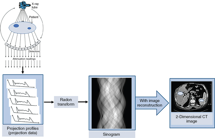
A CT image is reconstructed using a set of x-ray beam projections at different angles, that is, the x-ray tube and detectors rotate around the patient to collect attenuation readings, which are subsequently sent to a host computer that uses special programs (software) to reconstruct a two-dimensional (2D) image of the patient’s internal anatomy, using the projection data, or projections profiles (created by the detector electronics) as illustrated in Fig. 5.1. To arrive at the final 2D image, a number of digital signal processing techniques are used, such as for example, the Fourier transform (fast Fourier transform [FFT]), the Central Slice Theorem, also know as the Fourier Slice Theorem, and the Nyquist Theorem.
The mathematics of CT involves two problems: a forward problem and an inverse problem. In the forward problem, x-rays pass through the object at various angles to create projection data, the “raw data,” which represents the total attenuation of different structures in the object (various tissues in a patient). What is not known are the exact attenuation values of each of the structures along the path of x-rays. This is the second problem, the inverse problem, and it can be applied to determine the structures in the object using the projection data.
The mathematical tool used in the forward problem is the Radon transform, which creates an image that looks like an “x-ray film image” referred to as a sinogram (Radon transforms), as illustrated in Fig. 5.1. The next step involves converting the Radon transforms (sinograms) back into attenuation coefficients using the inverse Radon transform, to reconstruct a CT image of the patient’s internal anatomy. The CT inverse problem can be solved using several mathematical methods (Abbasi, 2020) as illustrated in Fig. 5.2. Two of these include the use of linear algebra methods and the use of frequency methods. The latter methods include algorithms such as the filtered back projection, iterative algorithms, and artificial intelligence based algorithms. The basic elements of both methods will be highlighted briefly in the rest of the chapter.

The remainder of this chapter will attempt to provide simple explanations of these complex mathematical topics. As image reconstruction is at the heart of the CT process, it is essential that technologists have a reasonable understanding of the basic image reconstruction principles that play a vital role in producing images that are used in the medical management of the patient. These methods are also a part of clinical protocols that guide the conduct of the examination.
In summary, the problem in producing a CT image is purely mathematical (the forward and inverse problems introduced earlier), and therefore mathematical solutions are needed to solve this problem. The description of the various approaches (computer programs [algorithms]) to creating CT images will begin with a very basic overview of the following mathematical terms that are commonly used in CT. These include algorithms, Fourier transform (FT), convolution, interpolation, and the Nyquist theorem.
Essential mathematical terminology
Algorithms
The algorithm is now common in radiology because computers are used in many imaging and non-imaging applications. The word “algorithm” is derived from the name of the Persian scholar, Abu Ja’Far Mohammed ibn Mûsâ Alkowârîzmî, whose textbook on arithmetic (c. 825 CE) significantly influenced mathematics for many years (Knuth, 1977). According to Knuth, an algorithm is “a set of rules or directions for getting a specific output from a specific input. The distinguishing feature of an algorithm is that all vagueness must be eliminated; the rules must describe operations that are so simple and well defined, they can be executed by a machine. Furthermore, an algorithm must always terminate after a finite number of steps.”
The solutions to mathematical problems in CT require image reconstruction algorithms, which are available as computer software, to reconstruct the image.
Fourier transform
The Fourier transform, which was developed by the mathematician Baron Jean-Baptiste-Joseph Fourier in 1807, is widely used in science and engineering. The FT is a useful analytical tool in mathematics, astronomy, chemistry, physics, medicine, and radiology. In radiology, the FT is used to reconstruct images of a patient’s anatomy in CT and also in magnetic resonance imaging (MRI).
To understand the FT, Bracewell (1989) presented an analogy with the act of hearing. Incoming sound waves that enter the ear are separated into different signals and intensities. These signals arrive at the brain and are rearranged to produce a perception of the original sound. Bracewell (1989) defined the FT as “a function that describes the amplitude and phases of each sinusoid, which corresponds to a specific frequency. (Amplitude describes the height of the sinusoid; phase specifies the starting point in the sinusoid’s cycle.)” In other words, the FT is a mathematical function that converts a signal in the spatial domain to a signal in the frequency domain (see Chapter 2).
The FT divides a waveform (sinusoid) into a series of sine and cosine functions of different frequencies and amplitudes. These components can then be separated. In imaging, when a beam of x-rays passes through the patient, an image profile denoted by f(x) is obtained. This can be expressed mathematically in the form of the Fourier series as follows:
The constants—a0, a1, b1, and so on—are called Fourier coefficients (Gibson, 1981) and can easily be calculated. Use of these Fourier coefficients makes it possible to reconstruct an image in CT.
Fourier central slice theorem
The Fourier central slice theorem is also referred to as the projection-slice theorem, or simply the central slice theorem. The mathematical basis is not within the scope of this chapter; however, the fundamental description of its use in CT is as follows: the projections obtained in CT as the x-ray beam passes through the patient are used to create images of the internal anatomy of the patient. When a FT (or more specifically the FFT, which reduces the number of computations required) is applied to these images, they are viewed as slices using the FFT of the 3D density of the internal anatomy of the patient. Subsequently, these slices can be interpolated to build up a complete FT of the 3D density. A further description of this will follow later in this chapter.
This theorem worked very well for second-generation CT scanners (see Chapters 1 and 4) that used parallel beam geometries CT; however, with the introduction of third-generation CT scanners with fan-beam and cone-beam geometries (see Chapters 1 and 4), the theorem had to be extended to address these geometries, using what is referred to as fan-beam and cone-beam image reconstruction (Zhao & Halling, 1995).
Nyquist theorem
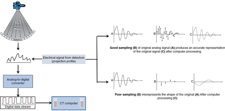
The Nyquist Theorem (developed by Harry Nyquist, an engineer at Bell Laboratories, about 100 years ago, as he explored the concept of digitizing sound) is also referred to as the Sampling Theorem (see Chapter 9) and is a vital part of digital signal processing, to digitize analog signals. This theorem is used today in CT whereby analog signals from the detectors are digitized (into zeros [0s] and ones [1s]) before they are sent to the CT host computer for processing (see Chapters 2 and 4).
A CT signal is obtained as shown in Fig. 5.3A. This analog signal (intensity profile from the patient which is a continuous signal) from the detectors must first be sampled and subsequently digitized by the analog-to-digital converter (ADC), which is an essential component of the Data Acquisition System (DAS) of the CT scanner. Sampling and digitization belong to the domain of digital signal processing (DSP) as described in Chapter 2. “The Nyquist theorem states that an analog signal waveform can be converted to digital format and be reconstructed without error from samples taken at equal time intervals if the sampling rate is equal to, or greater than, twice the highest frequency component in the analog signal” (Yourdictionary, 2020). In CT, this simply means that the sampling frequency, that is, the number of rays/cm in the fan beam, must be at least twice the highest frequency content in the signal. If the Nyquist criterion is not met, aliasing artifacts (streaks) will be seen on the CT image (see Chapter 9). Two examples of good and poor sampling are illustrated in Figure 5.3B. Poor sampling will result in aliasing artifacts (see Chapter 9).
Convolution
Convolution is a digital image-processing technique (see Chapter 2) used to modify images through a filter function (see Chapter 2). “The process involves multiplication of overlapping portions of the filter function and the detector response curve selectively to produce a third function which is used for image reconstruction” (Berland, 1987). (This will become clear during the discussion of the filtered back-projection algorithm.)
Interpolation
Interpolation is used in CT in the image reconstruction process and the determination of slices in spiral/helical CT imaging. Interpolation is a mathematical technique used to estimate the value of a function from known values on either side of the function.
For example, if the speed of an engine controlled by a lever increases from 40 to 50 revolutions per second when the lever is pulled down by 4 cm, one can interpolate from this information and assume that moving it 2 cm gives 45 revolutions per second. This is linear interpolation, which is the simplest method of interpolation. If known values of one variable, Y, are plotted against the other variable, X, an estimate of an unknown value of Y can be made by drawing a straight line between the two nearest known values.
The mathematical formula for linear interpolation is as follows:
where Y3 is the unknown value of Y (at X3) and Y2 and Y1 (at X2 and X1) are the nearest known values between which the interpolation is made (Gibson, 1981).
Image reconstruction from projections
As shown in Fig. 5.2, image reconstruction is a part of the solutions to the CT inverse problem. The sequence of events after the data are collected from the detectors is shown in Fig. 5.4. Although the older CT scanners collected data over 180 degrees, present-day CT scanners collect more attenuation data over 360 degrees to generate better-quality images. The image reconstruction algorithms, as they are referred to, are numerous and have been developed and subsequently modified to meet the requirements of the new generation of CT scanners.
Historical perspective
The history of reconstruction techniques dates back to 1917 when Radon developed mathematical solutions to the problem of image reconstruction from a set of its projections. He applied these techniques to gravitational problems. They were later used to solve problems in astronomy and optics, but they were not applied to medicine until 1961 (Fig. 5.5).

In his initial work, Hounsfield’s images were noisy as a result of his chosen reconstruction technique. Special algorithms (convolution back-projection algorithms) were soon introduced. These algorithms were developed by Ramachandran and Lakshminarayanan (Ram/Lak for short [1971]) and later used by Shepp and Logan (1974) to improve image quality and processing time.
Mathematical problem in CT
Consider an object, O, represented by an x-y coordinate system (Fig. 5.6). The spatial distribution of all attenuation coefficients, μ, is given by μ(x,y), which varies between points in the object. Suppose a pencil beam of x rays passes through the object along a straight path (arrow), and the intensity of the transmitted beam that falls on the CT detector is I. Then a projection is given by the line integral1 of μ(x,y):

By taking the negative logarithm, Equation 5.1 can be linearized to generate integral equations of the form

where T0(x) is the x-ray transmission at angle θ, which is a measure of the total absorption along the straight line in Figure 5.6. Tθ(x) is referred to as the ray sum, which is the integral of μ(x,y) along the ray.
The computational problem in CT is to find μ(x,y) from the ray sums for a sufficiently large number of beams of known locations that pass through the object, O. The beam geometries discussed in Chapter 4 ensure that every point in the object is scanned successively by a large set of ray sums Tθ(x).
A set of ray sums is referred to as a projection, which can be generated as shown in Fig. 5.7, as the x-ray tube and detector scan the object simultaneously. The ray AA´ is equal to x cos θ + y sin θ = d. The projection is given by P(θ,d):

where ds is the differential along the path length s.
To understand the meaning of a projection, consider the following case in which a beam of intensity Iin enters an object of thickness x:

The beam is attenuated according to the Beer’s law, as follows:

Because x, Iin, Iout, and e are known, μ can be calculated as follows:
The following case represents the situation in the patient:

Because x1 = x2 = x3... = xn,
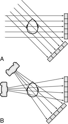
The problem in CT is to calculate all values for the μ terms for a large set of projections. Projections can be obtained through both parallel and fan beam geometries (Fig. 5.8). Hounsfield’s original CT scanner used parallel beam projections acquired through a 180-degree rotation.
Reconstruction algorithms
Image reconstruction from projections involves several algorithms to calculate all the μ terms in Equation 5.7 from a set of projection data. The algorithms applicable to CT include back-projection, iterative methods, and analytic methods.
Back-projection
Back-projection is a simple procedure that does not require much understanding of mathematics. Back-projection, also called the “summation method” or “linear superposition method,” was first used by Oldendorf (1961) and Kühl and Edwards (1963). Back-projection can be best explained with a graphical or numerical approach.
Consider four beams of x rays that pass through an unknown object to produce four projection profiles P1, P2, P3, and P4 (Fig. 5.9). The problem involves the use of these profiles to reconstruct an image of the unknown object (black dot) in the box. The projected datasets are back-projected (i.e., linearly smeared) to form the corresponding images BP1, BP2, BP3, and BP4. The reconstruction involves summing these back-projected images to form an image of the object.

The problem with the back-projection technique is that it does not produce a sharp image of the object and therefore is not used in clinical CT. The most striking artifact of back-projection is the typical star pattern that occurs because points outside a high-density object receive some of the back-projected intensity of that object (Curry et al., 1990).
Back-projection can also be explained using linear algebra, a branch of mathematics regarding linear equations, and concerns linear combinations. Linear algebra uses “arithmetic on columns of numbers called vectors and arrays of numbers called matrices, to create new columns and arrays of numbers. Linear algebra is the study of lines and planes, vector spaces and mappings that are required for linear transforms” (Brownlee, 2020).
The following back-projection can be explained using linear algebra with the following 2 × 2 matrix:

Four separate equations can be generated for the four unknowns, μ1, μ2, μ3, and μ4:
A computer can solve these equations very quickly.
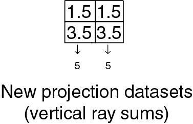
A numerical example might help give some insight into the calculations involved. Consider an object divided into four squares (2 × 2 matrix with four pixels).
Four projections are collected at four different known locations: 0, 45, 90, and 135 degrees.
To start, data are collected for four projections: 0, 45, 90, and 135 degrees.
- 1. The ray sum for the 0-degree projection on the left side is 1 (0 + 1).
- 2. The ray sum for the 0-degree projection on the right side is 5 (2 + 3).
- 3. The ray sums for the 45-degree projection are 0, 3 (2 + 1), and 3.
- 4. The ray sum for the 90-degree projection on the upper row is 2 (2 + 0).
- 5. The ray sum for the 90-degree projection on the lower row is 4 (3 + 1).
- 6. The ray sums for the 135-degree projection are 2, 3 (3 + 0), and 1.
These projection data—1, 5, 0, 3, 3, 2, 4, 2, 3, and 1—are then used systematically as defined by the algorithm to reconstruct the original image.
- 1. First guess: Place the data from the 0-degree projections into the matrix to obtain the first guess:

- 2. Second guess: Add the data from the 45-degree projections to the value of each square in the first guess:

- 3. Third guess: Add the data from the 90-degree projections to the value of each square in the second guess:

- 4. Fourth guess: Add the data from the 135-degree projections to the value of each square in the third guess:

The next step is to obtain the original matrix, as follows:


This is the original 2 × 2 matrix.
Iterative algorithms
Another approach to image reconstruction is based on iterative techniques. “An iterative reconstruction starts with an assumption (for example, that all points in the matrix have the same value) and compares this assumption with measured values, makes corrections to bring the two into agreement, and then repeats this process over and over until the assumed and measured values are the same or within acceptable limits” (Curry et al., 1990).
Techniques include the simultaneous iterative reconstruction technique, the iterative least-squares technique, and the algebraic reconstruction technique (Brooks & Di Chiro, 1976; Gordon & Herman, 1974). These techniques differ in the application of corrections to subsequent iterations. The algebraic reconstruction technique was used by Hounsfield in the first EMI brain scanner (Hounsfield, 1972) and is detailed here.
Consider the following numeric illustration:

- 1. Initial estimate: Compute the average of four elements and assign it to each pixel, that is, 1 + 2 + 3 + 4 = 10; 10/4 = 2.5

- 2. First correction for error (original horizontal ray sums minus the new horizontal ray sums divided by 2) = (3 − 5)/2 and (7 − 5)/2 = −2/2 and 2/2 = −1.0 and 1.0

- 3. Second estimate:
- 4. Second correction for error (original vertical ray sums minus new vertical ray sums divided by 2) = (4 − 5)/2 and (6 − 5)/2 = −1.0/2 and +1.0/2 = −0.5 and +0.5:


In the early years of CT use these iterative techniques were not used in commercial scanners because of the following limitations:
- 1. It is difficult to obtain accurate ray sums because of quantum noise and patient motion.
- 2. The procedure takes too long to generate the reconstructed image because the iteration can be done only after all projection datasets have been obtained, and because of the lack of computing power to solve these equations quickly.
- 3. To produce a “true” image, there should be more projection datasets than pixels. Therefore, diagonal projection datasets are taken to eliminate ambiguity.
Today, iterative reconstruction algorithms have resurfaced because of the availability of high-speed computing (Beister et al., 2012). The primary advantages of iterative image reconstruction algorithms are to reduce image noise (Beister et al., 2012; Hsieh et al., 2013; Kaza et al., 2014) and minimize the higher radiation dose (Fleischmann & Boas, 2011; McCollough et al., 2012) inherent in the filtered back-projection algorithm.
All major CT manufacturers offer iterative reconstruction algorithms as of 2014. For example, while GE Healthcare and Philips Healthcare offer Adaptive Statistical Iterative Reconstruction (ASiR), Model-Based Iterative Reconstruction (MBIR), and Iterative Model Reconstruction, Siemens Healthcare offers Image Reconstruction in Image Space (IRIS) and Sinogram Affirmed Iterative Reconstruction (SAFIRE). Toshiba Medical Systems, on the other hand, offers the Adaptive Iterative Dose Reduction (AIDR) iterative algorithm.
Iterative reconstruction algorithms are described in more detail in Chapter 6.
Analytic reconstruction algorithms
Analytic reconstruction algorithms were developed to overcome the limitations of back-projection and iterative algorithms and are used in modern CT scanners. Two analytic reconstruction algorithms are the Fourier reconstruction algorithm and filtered back-projection.
Filtered back-projection
Filtered back-projection is also referred to as the convolution method (Fig. 5.10) (a noteworthy point is that the projection slice theorem is the basis for this algorithm).
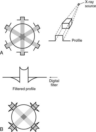
The projection profile is filtered or convolved to remove the typical starlike blurring that is characteristic of the simple back-projection technique.
The steps in the filtered back-projection method (see Fig. 5.10B) are as follows:
- 1. All projection profiles are obtained.
- 2. The logarithm of the data is obtained.
- 3. The logarithmic values are multiplied by a digital filter, or convolution filter, to generate a set of filtered profiles.
- 4. The filtered profiles are then back-projected.
- 5. The filtered projections are summed and the negative and positive components are therefore canceled, which produces an image free of blurring.
Major problems with the filtered back-projection algorithm include noise and streak artifact (Beister et al., 2012).
Fourier reconstruction
The Fourier reconstruction process is used in MRI but not in modern CT scanners because it requires more complicated mathematics than the filtered back-projection algorithm.
A radiograph can be considered an image in the spatial domain; that is, shades of gray represent various parts of the anatomy (e.g., bone is white and air is black) in space. With the Fourier transform, this spatial domain image—the radiograph represented by the function f(x,y)—can be transformed into a frequency domain image represented by the function F(u,v). This frequency domain image consists of a range of high to low frequencies. In addition, this image can be retransformed into a spatial domain image with the inverse Fourier transform (Fig. 5.11).

There are several advantages to this transformation process. First, the image in the frequency domain can be manipulated (e.g., edge enhancement or smoothing) by changing the amplitudes of the frequency components. Second, a computer can perform those manipulations (digital image processing). Third, frequency information can be used to measure image quality through the point spread function, line spread function, and modulation transfer function (Huang, 1999).
The Fourier slice theorem states that the Fourier transform of the projection of an object at angle θ is equal to a slice of the Fourier transform of the object along angle θ (Fig. 5.12).

The Fourier reconstruction consists of the following steps (Fig. 5.13):
- 1. The object to be scanned is represented by the function f(x,y).
- 2. Projection data are obtained from the object. A projection dataset for at least a 180-degree rotation is required for adequate reconstruction. These projections represent a spatial domain image.
- 3. Each projection is transformed into the frequency domain by the Fourier transform. This image must be converted into a clinically useful image.
- 4. Because CT scanners use a FFT developed specifically for digital implementation, the frequency domain image must be placed on a rectangular grid (see Fig. 5.13). This is accomplished by interpolation. The FFT requires that the pixels in the grid array be 2, 4, 8, 16, 32, 64, 128, 256, 512, 1024, and so on.
- 5. Finally, the interpolated image is transformed into a spatial domain image of the object through an inverse Fourier transform operation.

The Fourier reconstruction technique does not use any filtering because interpolation produces a similar result. Also, the 2D interpolation process may introduce artifacts if it is not conducted accurately; therefore, it is not used in CT.
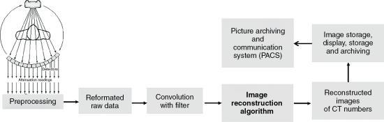
Types of data
Fig. 5.14 shows the data evolution from acquisition, reconstruction, and image display. Four data types are measurement data, raw data, filtered raw data or convolved data, and image data or reconstructed data.

Measurement data
Measurement data, or scan data, arise from the detectors. This dataset is subject to preprocessing to correct the measurement data before the image reconstruction algorithm is applied. Such corrections are necessary because of errors in the measurement data from beam hardening, adjustments for bad detector readings, or scattered radiation. If these errors are not corrected, they will cause poor image quality and generate image artifacts (see Chapter 9).
Raw data
Raw data are the result of preprocessed scan data and are subjected to the image reconstruction algorithm used by the scanner. These data can be stored and subsequently retrieved as needed.
Convolved data
The image reconstruction algorithm used by current CT scanners is the filtered back-projection algorithm, which includes both filtering and back-projection. Raw data must first be filtered with a mathematical filter, or kernel. This process is also referred to as the convolution technique. Convolution improves image quality through the removal of blur (Fig. 5.15). Figure 5.15A shows the degree of blurring present in an image before convolution. Figure 5.15B demonstrates image sharpening after convolution. Convolution kernels can only be applied to the raw data.
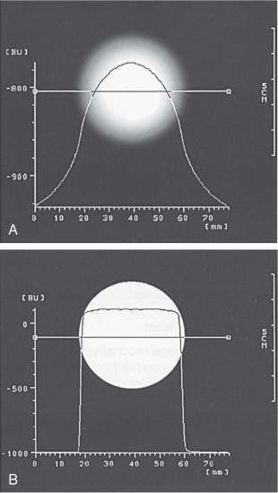
Image data
Image data, or reconstructed data, are convolved data that have been back-projected into the image matrix to create CT images displayed on a monitor. Various digital filters are available to suppress noise and improve detail (Fig. 5.16). Figure 5.16 shows the relationship between image noise and image detail of a standard algorithm, a smoothing algorithm, and an edge enhancement algorithm.

The standard algorithm is usually used before the previous algorithms, especially when a balance between image noise and image detail is mandatory. Smoothing algorithms (Fig. 5.17) reduce image noise and show good soft tissue anatomy; they are used in examinations where soft tissue discrimination is important to visualize very-low-contrast structures. Edge enhancement algorithms emphasize the edges of structures and improve detail but create image noise (see Fig. 5.17). They are used in examinations in which fine detail is important, such as inner ear, bone structures, thin slice, and fine pulmonary structures.
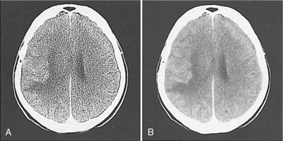
Image reconstruction in single-slice spiral/helical CT
The image reconstruction algorithms previously described apply to single-slice conventional CT (SSCT). In SSCT, the same filtered back-projection algorithm is used with an additional consideration. Because the patient moves continuously through the gantry for a 360-degree rotation, the reconstructed image will be blurred, so interpolation is necessary before the filtered back-projection is used. A planar section must first be computed from the volume dataset by using interpolation, after which images are generated with various interpolation algorithms. A more comprehensive description of these algorithms is presented in Chapter 12.
Image reconstruction in multislice spiral/helical CT
A notable difference between SSCT and multislice CT (MSCT) is that the latter uses multiple detector rows that cover a larger volume at an increased speed and therefore require new algorithms. In general, for CT scanners with four detector rows, MSCT algorithms have been developed to allow for the reconstruction of variable slice thicknesses and address the problems of increased volume coverage and speed of the patient table. This is made possible by spiral/helical scanning with interlaced sampling, longitudinal interpolation, and fan beam reconstruction with the filtered back-projection algorithm. These three major steps are described further in Chapter 12.
The new generation of MSCT scanners (those with 16 and greater detector rows) requires modified image reconstruction algorithms. These algorithms are very complex and beyond the scope of this textbook; however, a few foundational concepts relating to these algorithms are introduced in the next section and further elaborated in Chapter 11, which deals specifically with MSCT principles and concepts.
Cone-beam algorithms for multislice CT scanners
A number of image reconstruction algorithms have been developed for conventional “stop-and-go” (or “step-and-shoot”) CT scanners, SSCT scanners, and MSCT scanners with four detector rows.
There are several types of image reconstruction algorithms and specific beam geometries characteristic of the new CT scanners and these are described further in Chapter 12. Although conventional CT scanners use pencil beam and small fan beam geometries with the filtered back-projection image reconstruction algorithm, SSCT scanners use wide fan beam geometries. Here the image reconstruction algorithm is based on interpolation followed by filtered back-projection. MSCT scanners with four detector rows use a wider fan beam geometry (compared with SSCT scanners) and use a 2D reconstruction with interpolation and z-filtering, known as z-interpolation algorithms (Chen et al., 2003).
The algorithms for the SSCT and MSCT with four detector rows are referred to as spiral/helical fan beam approximation algorithms (Hu, 1999) simply because they are based on the fan beam geometry. According to Hein et al. (2003), the fan beam approximation algorithm “assumes that the source, detector, and slice of interest lie in the same plane, and that the projection of the slice of interest falls on a single detector row. This approximation is valid for small cone angles associated with one to four slice systems.” The cone angle is associated with cone-beam geometry (Flohr et al., 2005).
Cone-beam geometry
For a four-detector row MSCT scanner, the beam divergence from the x-ray tube to the outer edges of the detectors increases, as shown in Fig. 5.18. Such a beam is called a cone beam. Within the cone beam, the rays that will be measured by the detectors are tilted at an angle relative to the central plane (plane perpendicular to the long axis of the patient, the z-axis). This angle is called the cone angle.

As the number of detector rows increases from 4 to 16 to 64 and 320, the cone angle becomes larger. The larger cone angles cause problems where the beam divergence along the z-axis becomes greater. This results in the plane of interest (planar section of slice of interest) being projected onto several detector rows (Hein et al., 2003). This situation generates inconsistent data that will lead to cone-beam artifacts, such as streaking and density changes, both of which will have a negative effect on image quality.
Cone-beam algorithms
Fan beam approximation algorithms require that the data be consistent, that is, the x-ray beam from the tube to the detector and the section being imaged must be in the same plane. This is no longer the case for large cone angles characteristic of MSCT systems with larger than four detector rows. The fan beam approximation algorithms are not very accurate when used with the new generation of MSCT scanners, so other image reconstruction algorithms are needed. These algorithms are called cone-beam algorithms, and they have been developed to eliminate the cone-beam artifacts previously mentioned. One such popular algorithm is the adaptive multiple plane reconstruction algorithm (Bruening & Flohr, 2003).
Essentially, several cone-beam algorithms have become available for use with the new generation of MSCT scanners, and they basically fall into two classes: exact cone-beam algorithms and approximate cone-beam algorithms (Kalender, 2005). These algorithms are described further in Chapter 12, because the terminology for these new MSCT scanners is an important requirement for understanding cone-beam algorithms.
An overview of three-dimensional reconstruction techniques
The applications of 3D imaging are rapidly increasing (Calhoun et al., 1999; Cody, 2002; Dalrymple et al., 2005; Fishman et al., 2006; Logan, 2001; Udupa, 1999; Udupa & Herman, 2000). 3D imaging uses 3D surface and volumetric reconstruction. The algorithms for 3D imaging are based on those used in computer graphics and visual perception science. A 3D reconstruction technique for surface display (Fig. 5.19) is based on at least two processes, preprocessing and display, and consists of the following operations: interpolation, segmentation, surface formation, and projection (Cody, 2002; Philipp et al., 2003; Udupa & Herman, 2000; Zhang et al., 2011). 3D reconstruction techniques allow the user to “interactively visualize, manipulate, and measure large 3D objects on general purpose workstations” (Dalrymple et al., 2005; Fishman et al., 2006; Udupa & Herman, 2000).

3D reconstruction techniques are described in detail in Chapter 14.
Review questions
Answer the following questions to check your understanding of the materials studied.
- 1. Which of the following changes a time domain signal into a frequency domain signal?
- 2. A measure of the total absorption of x-rays along a straight line is referred to as:
- 3. The basic problem in CT is to calculate:
- 4. The horizontal ray sums for the pixels shown below are:

- 5. The back-projection technique results in:
- 6. CT scanners now use the:
- 7. Image data are obtained:
- 8. The first operation to which raw data are subjected is referred to as:
- 9. Which of the following belongs to the class of analytic algorithms for CT?
- 10. Which of the following uses a digital filter to modify an image matrix?
References
Abbasi N.M. The application of Fourier analysis in solving the computed tomography (CT) inverse problem 2020; Fullerton Master of Science (MSc) Project in Applied Mathematics at CSUF Mathematics department in 2008. California State University.
Beister M, Kolditz D. & Kalender W.A. Iterative reconstruction methods in X-ray CT Physica Medica 2, 2012;28: 94-108 doi:10.1016/j.ejmp.2012.01.003.
Berland L.L. Practical CT: Technology and techniques 1987; Raven Press New York.
Bracewell R. The Fourier transform Scientific American 1989;260: 86-95.
Brooks R.A. & Di Chiro G. Principles of computer assisted tomography (CAT) in radiographic and radioisotopic imaging Physics in Medicine and Biology 1976;21: 689-732.
Brownlee, J. (2020). A gentle introduction to linear algebra. Retrieved from https://machinelearningmastery.com/gentle-introduction-linear-algebra/. Accessed October, 2020.
Bruening R. & Flohr T. Protocols for multislice CT—4 and 16 row applications 2003; Springer Verlag New York.
Calhoun P.S, Kuszyk B.S, Heath D.G, Carley J.C. & Fishman E.K. Three-dimensional volume rendering of spiral CT data: Theory and method Radiographics 1999;19: 745-764.
Chen, S. (2019). Mathematical medicine: Computed tomography (CT scans). Retrieved from https://medium.com/@sullyfchen/mathematical-medicine-computed-tomography-ct-scans-f2a762f398e7. Accessed October 2020.
Chen L, Liang Y. & Heuscher D.J. General surface reconstruction for cone beam multislice spiral computed tomography Medica Physica 2003;30: 2804-2812.
Cody D.D. AAPM/RSNA physics tutorial for residents: Topics in CT. Image processing in CT Radiographics 2002;22: 1255-1268.
Curry T.S. III, Dowdy J.E, Murry R.C. & Jr. Christensen’s physics of diagnostic radiology 4th ed. 1990; Lea & Febiger Philadelphia, PA.
Dalrymple N.C, Prasad S.R, Freckleton M.W. & Chintapalli K.N. Introduction to the language of three-dimensional imaging with multidetector CT Radiographics 2005;25: 1409-1428.
Faridani, A. (2020). Introduction to the mathematics of computed tomography. Dept. of Mathematics, Oregon State University, Corvallis, OR. Retrieved from http://library.msri.org/books/Book47/files/faridani.pdf. Accessed October 2020.
Fishman E.K, Ney D.R, Health D.G, Corl F.M, Horton K.M. & Johnson P.T. Volume rendering versus maximum intensity projection in CT angiography: What works best, when, and why Radiographics 2006;26: 905-922.
Fleischmann D. & Boas F.E. Computed tomography: Old ideas and new technology European Radiology 3, 2011;21: 510-517 doi:10.1007/s00330-011-2056-z.
Flohr T.G, Schaller S, Stierstorfer K, Bruder H, Ohnesorge B.M. & Schoepf U.J. Multi-detector row CT systems and image reconstruction techniques 2005; Radiology 756-773.
Gibson C. The facts on file dictionary of mathematics 1981; Facts on File New York.
Gordon R. & Herman G.T. Three-dimensional reconstruction from projections: A review of algorithms International Review of Cytology 1974;38: 111-123.
Hein I, Taguchi K, Silver M.D, Kazama M. & Mori I. Feldkamp-based cone beam reconstruction for gantry-tilted helical multislice CT Medica Physica 2003;30: 3233-3242.
Herman G.T. Fundamentals of computerized tomography: Image reconstruction from projections 2009; Springer New York.
Hounsfield, G. H. (1972). A method of and apparatus for examination of a body by radiation such as X or gamma radiation. British Patent Office, Patent No. 1283915.
Hsieh J, Nett B, Zhou Y, Sauer K, Thibault J.B. & Bouman C.A. Recent advances in CT image reconstruction Current Radiology Reports 1, 2013;1: 39-51 10.1007/s40134-012-0003-7.
Hu H. Multislice helical CT: Scan and reconstruction Medica Physica 1, 1999;26: 5-18.
Huang H.K. PACS: Basic principles and applications 1999; Wiley-Liss New York.
Kak A.C. & Slaney M. Principles of computerized tomographic imaging 1999; IEEE Ed New York.
Kharfi F. Mathematics and physics of computed tomography (CT): Demonstrations and practical examples 2013; IntechOpen Ltd London, UK.
Kalender W.A. Computed tomography: Fundamentals, system technology, image quality, applications 2005; GWA Erlangen, Germany.
Kaza R.K, Platt J.F, Goodsitt M.M., et al. Emerging techniques for dose optimization in abdominal CT Radiographics 1, 2014;34: 4-17 10.1148/rg.341135038.
Knuth D.E. Algorithms Scientific American 1977;236: 63-80.
Kühl D.E. & Edwards R.Q. Image separation radioisotope scanning Radiology 1963;80: 653-661.
Logan L. Seeing the future in three dimensions Radiologic Technology 2001;15: 483-487.
McCollough C.H, Chen G.H, Kalender W., et al. Achieving routine submillisievert CT scanning: Report from the summit on management of radiation dose in CT Radiology 2, 2012;264: 567-580.
Natterer F. The mathematics of computerized tomography 1986; Wiley and Sons and Stuttgart: BG Teubner New York.
Oldendorf W.H. Isolated flying spot detection radio-density discontinuities displaying the internal structural pattern of a complex object IEEE Transactions on Biomedical Engineering 1961;8: 68-72.
Parker D.L. & Stanley J.H. Glossary T.H. Newton & D.G. Potts. Glossary radiology of the skull and brain: Technical aspects of computed tomography 1981; Mosby St. Louis, MO.
Philipp M.O, Kubin K, Mang T, Hörmann M. & Metz V.M. Three-dimensional volume rendering of multidetector-row CT data: Applicable for emergency radiology European Journal of Radiology 2003;48: 33-38.
Ramachandran G.N. & Lakshminarayanan A.V. Three-dimensional reconstructions from radiographs and electron micrographs: Application of convolution instead of Fourier transforms Proceedings of the National Academy of Sciences of the United States of America 1971;68: 2236-2240.
Seeram E. Computed tomography technology 2001; WB Saunders Philadelphia, PA.
Shepp L.A. & Logan B.F. The Fourier reconstruction of a head section IEEE Transactions on Nuclear Science 1974;21: 21-43.
Udupa J.K. Three-dimensional visualization and analysis methodologies: A current perspective Radiographics 1999;19: 783-803.
Udupa J.K. & Herman G.T. 3D imaging in medicine 2000; CRC Press Boca Raton, FL.
Yourdictionary. (2020). Nyquist-theorem definitions. Burlingame, CA: LoveToKnow Corp. Retrieved from https://www.yourdictionary.com/nyquist-theorem. Accessed October, 2020.
Zhao S.R. & Halling H. A new Fourier transform method for fan beam tomography Nuclear Science Symposium and Medical Imaging Conference Record 1995;2: 1287-1291.
Zhang Q, Eagleson R. & Peters T.M. Volume visualization: A technical overview with a focus on medical applications Journal of Digital Imaging 4, 2011;24: 640-664.
Bibliography
Cho Z.H. & Ahn I.S. Computer algorithms for the tomographic image reconstruction with X-ray transmission scans Computers and Biomedical Research 1975;8: 8-25.
Fishman E.K, Magid D, Ney D.R., et al. Three-dimensional imaging Radiology 1991;181: 321-337.
Gabor H.T. Image reconstruction from projections 1980; Academic Press New York.
Kalender W.A, Seissler W, Klotz E. & Vock P. Single-breath-hold spiral volumetric CT by continuous patient translation and scanner rotation Radiology 1989;173: 414-419.
Strong A.B, Lobregt S. & Zonneveld F.W. Applications of three-dimensional display techniques in medical imaging Journal of Biomedical Engineering 1990;12: 233-238.