6: Iterative and deep learning reconstruction basics
Learning objectives
On completion of this chapter, you should be able to:
- 1. outline the assumptions made to derive the filtered back-projection (FBP) algorithm.
- 2. list four strategies to reduce noise in CT imaging.
- 3. state three categories of iterative reconstruction (IR) algorithms available from CT manufacturers.
- 4. describe three steps in a typical IR process without modeling.
- 5. state the meaning of the term “modeling” and list three models used in IR algorithms.
- 6. identify the points where these models are applied during the CT image reconstruction process.
- 7. state three goals of using IR algorithms in CT.
- 8. provide examples of various IR algorithms available from CT manufacturers.
- 9. define Artificial Intelligence (AI) and its subsets, Machine Learning (ML) and Deep Learning (DL).
- 10. describe how a conceptual framework of the training phase of a DL reconstruction engine works.
- 11. describe briefly how the trained DL reconstruction is applied in clinical practice.
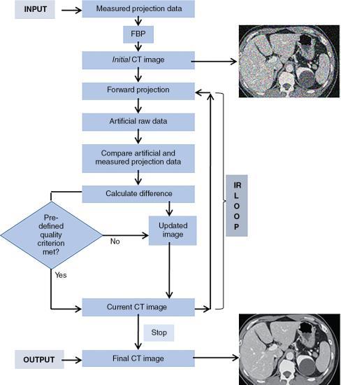
In Chapter 5, image reconstruction algorithms for computed tomography (CT) were described in general, including a numerical illustration of the first iterative reconstruction (IR) algorithm used by Dr. Godfrey Hounsfield (1973), the inventor of CT. He shared the 1979 Nobel Prize in Medicine and Physiology with Professor Allan Cormack, a physics lecturer at the University of Cape Town, South Africa. The filtered back-projection (FBP) algorithm, an early analytical reconstruction algorithm, was also described in Chapter 5. It has been the major reconstruction algorithm used in CT since the 1970s. The basic framework of the FBP algorithm is shown in Fig. 6.1. Essentially, the measured projection data (raw data) are subject to calibrations, corrections, and log conversion, and so on, followed by convolution filtering and back-projection (two key features of the FBP algorithm) to produce an image from which a diagnosis can be made.

The FBP algorithm is well recognized for its speed and “closed-form solution” (Hsieh, 2008), which is “available from a single pass over the acquired data” (Thibault, 2010). The FBP algorithm, however, has several limitations, including image noise and artifact creation (Hsieh et al., 2013; Thibault, 2010). While the noise problem can be overcome by increasing the milliamperes (mA) for the examination, radiation dose to the patient becomes a real challenge. This situation becomes more pronounced in low-dose CT examinations, in an effort to adhere to the “as low as reasonably achievable” (ALARA) philosophy of the International Commission on Radiological Protection. This philosophy tries to ensure that the lowest possible dose is used without compromising the diagnostic quality of the image.
Assumptions made to derive the FBP algorithm
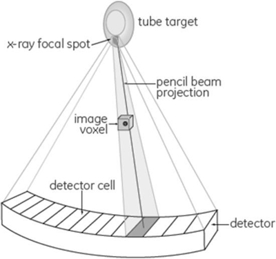
The problems with the FBP algorithm are due to several “idealized” assumptions made when deriving the algorithm. Fig. 6.2 has been used by Hsieh (2008) to illustrate the nature of these assumptions, which include:
- 1. The x-ray focal spot is a point source.
- 2. The size and shape of each detector cell is not taken into consideration.
- 3. “All x-ray photon interactions are assumed to take place at a point located at the geometric center of the detector cell, not across the full area of the detector cell.”
- 4. A pencil beam is used to “represent the line integral of the attenuation coefficient along the path” as shown in Fig. 6.2.
- 5. The size and shape of the voxels are described as “infinitely small points located on a square grid.”
- 6. The projection data are accurate and not affected by x-ray photon statistical changes and electronic noise.
The above assumptions of the CT system have been used successfully to derive the FBP algorithm. Such a CT system model “clearly does not represent physical reality” (Hsieh et al., 2013); therefore, other algorithms that model the CT system accurately are needed. These algorithms must consider accurate modeling of the CT system optics, the noise (noise model), and the image properties (image model). The highlights of modeling will be described later in the chapter. This is an important point to note, as accurate modeling results in improvements in image quality and noise reduction when compared with the FBP analytical algorithm.
Noise reduction techniques
The increasing use of CT has resulted in a corresponding increase in radiation dose to the patient and concerns about the potential biological effects of radiation exposure from CT examinations (Brenner & Hall, 2007; Pearce et al., 2012). Subsequently, these concerns have resulted in increasing awareness of various efforts to reduce the dose to the patient in CT scanning (Seeram, 2014; Seeram 2018).
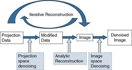
It is well known that the use of low-dose techniques can produce noisy images; therefore, it is essential to consider various approaches to noise reduction, especially in low-dose CT imaging. Fig. 6.3 shows four strategies to reduce the noise during CT image reconstruction. These include projection space denoising, analytical FBP denoising using standard reconstruction kernels (see Chapter 5), image space denoising, and the use of iterative reconstruction (IR) (Ehman et al., 2014). Whereas image space denoising and FBP-based analytic reconstruction use digital filters (e.g., smoothing filters, edge enhancement filters; see Chapter 2), projecting space denoising (filtering before image reconstruction) uses photon statistics to reduce noise through a statistical noise model or adaptive noise filtering (Ehman et al., 2014)
IR algorithms have been developed to reduce image noise in low dose CT, and at the same time to preserve image quality (namely, spatial resolution and low-contrast detectability [LCD]) and reduce artifacts due to the presence of metal implants, beam-hardening effects, and photon starvation (Ehman et al., 2014). These artifacts (and more) are common when using the traditional FBP algorithm (Hsieh et al., 2013; Zeng & Zamyatin, 2013).
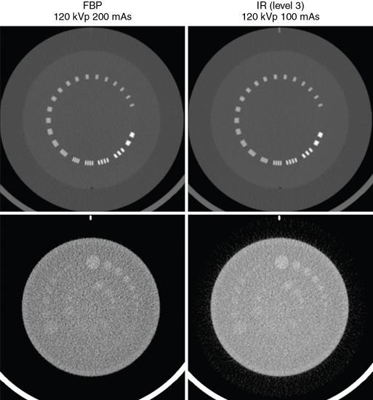
The fundamental differences between the FBP and IR algorithms are illustrated in Fig. 6.4.
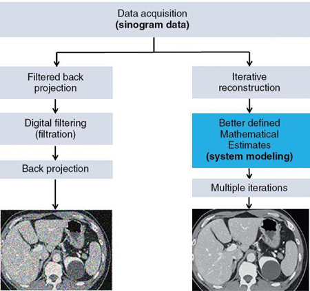
IR algorithms use better defined mathematical estimates (modeling) and multiple iterations to produce images with less noise at low dose exposures compared with the FBP algorithm. It is visually clear that the FBP image is much noisier than the IR image. The word iteration simply refers to a calculation process that uses a series of operations repeated several times.
There are several IR algorithms commercially available from CT scanner manufacturers, based on different physical methods and concepts. These algorithms must consider accurate modeling of the CT system optics, noise (noise model), and the image properties (image model).
In generally, IR algorithms differ in the way the measured projection data and the artificial raw data are compared and the method in which correction is applied to the current estimate.
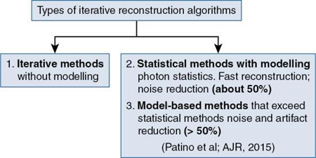
IR algorithms have been placed in the following three categories, as illustrated in Fig. 6.5:
IR algorithms without modeling: Fundamental concepts
A generalized or typical IR process is illustrated in a flowchart in Fig. 6.6, and consists of the following steps:
- 1. During scanning, iterative reconstruction acquires measured projection data and then reconstructs the data using the standard FBP algorithm to produce an initial image estimate.
- 2. The initial image estimate then is forward projected to create simulated projection data (artificial raw data) that are subsequently compared with the measured projection data.
- 3. The algorithm then determines differences between the two sets of data to generate an updated image that is back-projected on the current CT image; this minimizes the difference between the current CT image and the measured projection data.
- 4. The user must evaluate image quality based on a predetermined criterion included in the algorithm.
- 5. If the image quality criterion is not met, the iteration process repeats several times in an iterative cycle until the difference is considered sufficiently minimal.
- 6. The final CT image matches the selected quality criteria after the termination of the iterative cycle.
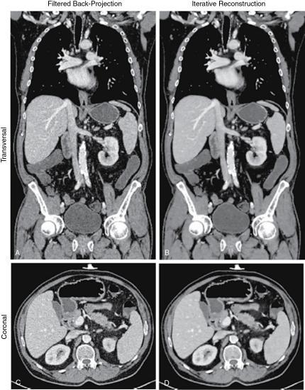
A comparison of images reconstructed using FBP and an IR algorithm is shown in Fig. 6.7.
The accuracy of the estimate mentioned previously depends on what is referred to as modeling the CT system acquisition components and the object being imaged. These will be briefly described in the following section.
Modeling approaches in IR algorithms: An overview
The term modeling is used to refer to the characteristics of the CT imaging system and the imaged object, and includes what has been popularly referred to as system optics (optics model), noise statistics (noise model), and object and physics models. These different system models are illustrated in Fig. 6.8, where the points to which they are applied during the CT IR process are shown.
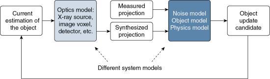
Whereas the optics model or system optics addresses the x-ray source, image voxel, and detectors, and so on, the noise model takes into consideration the x-ray photon statistics (x-ray flux at the source and detector). The object model, on the other hand, deals with radiation attenuation through the patient, whereas the physics model examines the physics of CT data acquisition. The interested reader should refer to Beister et al. (2012) and Hsieh et al. (2013) for a more detailed account of these models.
Whereas some IR algorithms model the system optics, others model the system noise statistics, physics, and objects. As noted by Hsieh et al. (2013), a “fully modeled IR is mor computationally intensive than analytical reconstruction methods.” Furthermore, Hsieh (2008) also points out that “the computational intensity on the modeling of the noise portion of the system is not nearly as big as the modeling of the system optics. Therefore, by focusing first on the modeling of the noise properties and the scanned object, we provide significant benefit for those examinations that may experience limitations due to noise in the reconstructed images, as a result of lower dose exams, large patients, thinner slices, etc. Phrased differently, we gain the dose benefit by lowering the noise in the reconstructed images, so that the scanning technique can be reduced with equivalent noise.”
Iterative methods without modeling compute an initial estimate of the image from the projection data set (using the FBP image), subsequently improving the image (current estimate) using several iterations (a calculation process using a series of operations repeated several times) (Patino et al., 2015).
Statistical IR methods
Statistical methods with modeling, on the other hand, use x-ray photons (photon counting statistics) during the IR process. Iterative statistical reconstruction algorithms can operate in the projection raw data domain (sonogram domain), in the image domain, and during the process of IR (Beister et al., 2012). With this notion in mind, General Electric (GE) Healthcare (Waukesha, WI) developed and introduced modeling iterative algorithms such as Adaptive Statistical Iterative Reconstruction (ASiR); ASiR-V; and Veo (fully model-based IR algorithm). (Bartak, 2020; Chen et al., 2017; Gordic et al., 2014; Irwan et al., 2011; Shin et al., 2020; Smith, 2013; Suzuki, 2017; Toshiba Medical Systems, 2015) state that ASiR “selectively identifies and removes noise from the low-dose CT images. It applies mathematical models to correct the image data by changing the photon statistics in X-ray attenuation. Noise is iteratively reduced in the image domain”. Additionally, explain that “ASIR-V is the vendor’s third-generation IR algorithm and replaces its first-generation algorithm, ASiR, on newer CT scanners. ASIR-V contains improved noise and object modeling compared with ASIR. It also applies parts of the physics model used in the vendor’s model-based algorithm (Veo, GE Healthcare) while excluding complex system optics in the modeling process. As a consequence, the image noise reduction potential of ASIR-V is lower than that of the model-based algorithm. However, its reconstruction time is substantially reduced, which is one of the major limitations for clinical use of model-based algorithms.”
Hybrid IR methods
Another class of IR algorithm that has been discussed in the CT literature is referred to as Hybrid IR. These algorithms combine IR and the FBP algorithm (den Harder et al., 2015). Examples of these include Adaptive Statistical Iterative Reconstruction (ASiR, GE Healthcare), Adaptive Iterative Dose Reduction 3D (AIDR 3D, Canon Medical Systems), Iterative Reconstruction in Image Space (IRIS, Siemens Healthineers), Sinogram-Affirmed Iterative Reconstruction (SAFIRE, Siemens Healthineers), Advanced Modeled Iterative Reconstruction (ADMIRE, Siemens Healthineers), and iDose4 (Philips Healthcare).
Model-based IR methods
As early as 2012, Beister et al. (2012), provided a description of model-based IR methods as follows: “...model-based methods try to model the acquisition process as accurately as possible. The acquisition is a physical process in which photons with a spectrum of energies are emitted by the focus area of the anode of the x-ray tube. Subsequently, they travel through the object and are either registered within the area of the detector pixel, scattered outside of the detector, or are absorbed by the object. The better the forward projection is able to model this process, the better the artificial image can be matched to the acquired raw data. Better matching artificial raw data leads to better correction terms for the next image update step and, in consequence to an improved image quality in the reconstruction data.”
Statistical and model-based methods are outside the scope of this book. The interested reader should refer to the paper by Beister et al. (2012) for a comprehensive description of the core principles of these two methods. A graphic illustration of the statistical iterative reconstruction algorithm (ASiR) and a model-based IR algorithm (Veo compared with the FBP analytical reconstruction algorithm) is shown in Fig. 6.9.
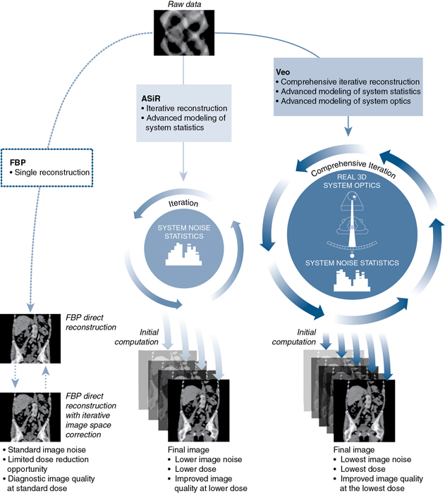
Recall that the goals of IR algorithms compared with the FBP algorithm are to improve image quality (namely, spatial resolution or sharpness of the image), reduction of noise, better low-contrast detectability (LCD), and artifact reduction. Such image quality improvement is shown in Fig. 6.10. This image quality improvement and reduction of dose depend on accurate modeling. For the improvement of image quality, it is important that the system optics are modeled accurately in the reconstruction process. For reduced dose, better LCD, and artifact reduction, it is mandatory that the noise statistics, the physics, and the object are modeled accurately in the reconstruction process.
Examples of IR algorithms from CT vendors
Several IR algorithms are currently available from major CT vendors such as General Electric (GE) Healthcare, Siemens Healthineers, Philips Healthcare, and Canon Medical Systems (formerly Toshiba Medical Systems). Each vendor offers propriety algorithms that provide improved image quality and noise reduction in low-dose CT imaging (dose reduction) compared with the FBP algorithm. Examples of these IR algorithms are listed in Table 6.1.
| CT Vendor | IR Algorithm | Acronym and Type |
|---|---|---|
| GE Healthcare | Adaptive Statistical Iterative Reconstruction | ASiR – Statistical |
| GE Healthcare | Veo Model-Based Iterative Reconstruction (with optimal use of statistical modeling) | Veo – Model Based |
| GE Healthcare | ASIR-V (includes advanced noise and object models with some physics modeling) | ASIR-V – Hybrid |
| Siemens Healthineers | Image Reconstruction in Image Space | IRIS – Hybrid |
| Siemens Healthineers | Sinogram-Affirmed Image Reconstruction | SAFIRE – Hybrid |
| Siemens Healthineers | Advanced Modeled Iterative Reconstruction | ADMIRE – Model Based |
| Philips | iDose (Iterative processing in projection [sinogram] and image domains) | iDose – Hybrid |
| Canon Medical Systems | Adaptive Iterative Dose Reduction | AIDR |
| Canon Medical Systems | Adaptive Iterative Dose Reduction 3D | AIDR 3D |
Furthermore, a literature review on the performance evaluation of these IR algorithms between 2012 to 2015 (Qiu & Seeram, 2016) concluded that “the results share the general consensus that IR algorithms do faithfully reduce radiation dose and improve image quality in CT examinations, when compared with the FBP algorithm. The use of IR algorithms definitively reduces objective image noise even at reduced radiation dose levels, while subjective image quality, in terms of spatial resolution and low contrast detectability, is improved or preserved with the use of IR algorithms as long as the radiation dose is not reduced excessively. However, the use of IR algorithms of excessively high iteration levels should be avoided, as the produced smoothing effect can negatively impact the subjective image quality. The use of IR algorithms may also be unable to preserve image detail in denser structures such as bone, although further research may be needed to validate this observation. With the rapid improvement in technology, IR algorithms will likely become the preferred CT image reconstruction method in the foreseeable future.” Today, IR algorithms have become commonplace in CT image reconstruction.
Deep learning reconstruction: An artificial intelligence-based approach-a new era
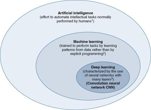
Artificial Intelligence (AI) is gaining widespread attention in healthcare and especially in medical imaging. One definition of AI given in Chapter 1 is that AI is the “effort to automate intellectual tasks normally performed by humans” (Chollet, 2018). As noted by Chartrand (2017), AI is “devoted to creating systems to perform tasks that ordinarily require human intelligence.” There are two subsets of AI, Machine Learning (ML), and Deep Learning (DL) which is a subset of ML, as illustrated in Fig. 6.11. Whereas ML is the use of algorithms that “are trained to perform tasks by learning patterns from data rather than by explicit programming” (Erickson et al., 2017), DL uses algorithms that are “characterized by the use of neural networks with many layers” (Chartrand et al., 2017). Furthermore, DL is based on the use of “a special type of artificial neural network (ANN) that resembles the multilayered human cognition system” (Lee et al., 2017). Additionally, the neural network many layers refer to “layers of mathematical equations and millions of connections and parameters that get trained and strengthened based on the desired output” (Hsieh et al., 2019).
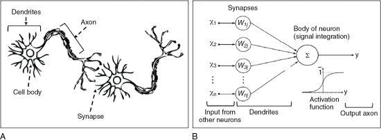
Humans think through the use of a complex network of real neurons (units of the nervous system) that make use of chemical and electrical signals. The conceptual difference between real neurons and artificial neurons is illustrated in Fig. 6.12. As shown in Figure 6.12A, the neuron is made up of a cell body, dendrites, axons, and synapses, and incoming signals are transmitted from one neuron to the next via synapses. In Figure 6.12B, the ANN is characterized by interconnected artificial neurons, where “each artificial neuron implements a simple classifier model that outputs a decision signal based on the weighted sum of evidences. Hundreds of these basic computing units are assembled together to establish the ANN. The weights of the network are trained by a learning algorithm, such as back propagation, where pairs of input signals and desired output decisions are presented, mimicking the condition where the brain relies on external sensory stimuli to learn to achieve specific tasks” (Lee et al., 2017). The elements of AI, including DL will be discussed further in Chapter 20.
Deep learning CT image reconstruction: Basic concepts
DL algorithms are now being applied to CT image reconstruction, which has been referred to as Deep Learning Reconstruction (DLR), or Deep Learning Image Reconstruction (DLIR). The ultimate goal of developing DLR is to provide improved image quality, dose performance, and reconstruction speed compared to previous image reconstruction algorithms, especially in low-dose CT scanning (Jensen et al., 2020). Two are currently available from CT vendors, Canon Medical Systems (Boedeker, 2019) and General Electric (GE) Healthcare (Hsieh et al., 2019) and were approved by the Food and Drug Administration in 2019. While Canon’s DLR CT reconstruction algorithm is referred to as the Advanced Intelligent Clear-IQ Engine (AiCE) DLR algorithm, the DLR algorithm from GE is referred to as TrueFidelity.
Limitations of FBP and IR algorithms
In Fig. 6.13, the influence of low-dose CT and the choice of the image reconstruction algorithm on image quality is illustrated. It is clear that in a high-dose CT situation, using the FBP algorithm the image quality is excellent; however, in a low-dose CT with the FBP algorithm, the image quality is poor. The solution to this problem is to use IR algorithms to provide improved image quality (compared to the low-dose FBP situation) using low-dose CT. IR delivers less image noise and artifact, “however, the smoothing artifact imparts a plastic-like, blotchy image appearance that has been observed in all iterative reconstructions particularly at higher levels. The modified appearance is considered a limitation of these techniques, and it affects the evaluation of CT scan images and, arguably, the interpretation of imaging findings” (Kim et al., 2019).
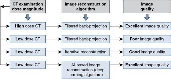
In an effort to provide excellent image quality using low dose CT, DLR algorithms have been introduced into the domain of CT image reconstruction. This development has often been referred to as a new era in CT image reconstruction (Hsieh et al., 2019).
Generalized framework for deep learning reconstruction
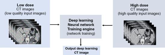
The location of a DL neural network training engine in CT is illustrated in Fig. 6.14. There are several types of deep learning neural networks, or deep neural network (DNN) for short, that are used for different purposes. For example, the Convolutional Neural Networks (CNNs) are neural networks that are used “primarily for classification of images, clustering of images and object recognition. CNNs enable unsupervised construction of hierarchical image representations. CNNs are used to add much more complex features to it so that it can perform the task with better accuracy” (Shukla & Iriondo, 2020). CNNs are not within the scope of this book; however, Do et al. (2020) provides a very brief description of a CNN as follows: “CNN is one of the artificial neural networks that can be characterized by a convolutional layer, which differs from other neural networks. A typical CNN is composed of a convolutional layer, a pooling layer, and a fully connected layer. The convolutional layer is the core of a CNN. In mathematical terms, “convolution” refers to the mathematical combination of two functions to produce a third function. When used in a CNN, convolution means that a kernel (or filter = small matrix) is applied to the input data to produce a feature map” (see Chapter 2 for the basics of convolution). CNNs have been applied exclusively in CT image reconstruction for low-dose computed tomography (LDCT) image denoising, and have been labelled DLIR (Chen et al., 2017; Kang et al., 2018; Shan et al., 2018).
In general, there are at least three phases for deep learning image reconstruction in CT (Hsieh et al., 2019) shown in Fig. 6.15: (1) design phase, (2) training and optimization phase, and (3) verification phase. Only the latter two will be highlighted in this chapter

Training and optimization
As seen, in Figure 6.14, both low-dose CT images created from the low-dose CT sinogram as well as high-dose CT images created from the high-dose sinogram (obtained from training data sets) are sent into the DL reconstruction (DLR) training engine where “learning” of features of the image occurs, and image parameters are adjusted, to provide an output image.
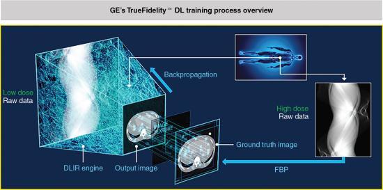
The training phase for GE’s TrueFidelity (Fig. 6.16) involves the input of a “low dose sinogram through the Deep Neural Network and comparing the output image to a ground truth image – a high dose version of the same data. These two images are compared across multiple image parameters such as image noise, low contrast resolution, low contrast detectability, noise texture, etc. The output image reports the differences to the network via backpropagation which then strengthens some equations and weakens others and tries again. This process is repeated till there is accuracy between the output image and the ground truth image” (Hsieh et al., 2019). Additionally:
- • The DL neural network training engine uses thousands of ground truth training data sets to create a mathematically exact ground truth CT image (reference image). In deep learning, the term is used to check the accuracy of the deep leaning algorithm results using factual data (objective data) fed into the DL engine.
- • The output CT image is then compared with the ground truth image (reference image) on image quality metrics such as, for example, image noise, spatial resolution, contrast resolution, low contrast detectability, noise texture, CT number accuracy, and anatomical features, to check for differences. The engine repeats the “learning” process until the output CT image matches the ground truth image (reference image) (Hsieh et al. 2019).
The training phase for Canon’s AiCE, illustrated in Fig. 6.17, involves the following elements (Lenfant et al., 2020; Boedeker, 2019):
- • First, a full dose CT sinogram is reconstructed by the model-based IR (MBIR) algorithm and a hybrid-IR algorithm using different scan conditions to create reference data sets (high-quality output and a low-quality input, respectively). These are fed into the CNN, where “learning” of features of the image occurs and image parameters (such as noise, spatial and contrast resolution, low contrast detectability, noise texture, and so on) are adjusted, to provide an output image.
- • Secondly, the DLR engine applies mathematical techniques to determine the amount of error (estimation error) between the output image and the reference datasets (ground truth reference) from which high-dose reference images are created from thousands of phantom and patient images using high tube current and the MBIR algorithm, and
- • Thirdly, the output image and the reference image are compared using the estimation error, and the CNN acts to decrease any “discrepancy” through the use of forward-backward propagation (Table 6.2) to obtain optimization (Lenfant et al., 2020; Boedeker, 2019).

| Terms/Concepts | Brief Descriptions |
|---|---|
| Ground Truth | A term used in various fields to refer to data and/or methods related to a greater consensus or to reliable values/aspects that can be used as references. In deep learning (DL), it usually refers to “correct labels” prepared by experts. |
| Data Curation | Organization and integration of data collected from various sources to add value to the existing data. Data curation includes all the processes necessary for principled and controlled data creation, maintenance, and management. Medical imaging data curation may include data anonymization, checking the representative of the data, unification of data formats, minimizing noise of the data, annotation, and creation of structured metadata such as clinical data associated with imaging data. |
| Data Augmentation | Acquiring large amounts of good-quality data is often difficult in clinical radiology. Data augmentation is an approach that alters the training data in a way that changes the data representation while keeping the label the same. It provides a way to artificially expand a dataset and maximize the usefulness of a well-curated image dataset. Popular augmentations of image data include blurring or skewing an image, modifying the contrast or resolution, flipping or rotating the image, adjusting zoom, and changing the location of a lesion |
| Training, Validation, and Test Data | Training data are used to train and optimize the parameters of the model. The validation data are used to monitor the performance of the model during the training and to search for the best model. The test data are used to finally evaluate the performance of the developed model. |
| Parameter versus Hyperparameter | A parameter refers to a variable that is automatically adjusted during the model training. A “hyperparameter” is a variable used to design the deep learning model and is a variable to be set before training the model. |
| CNN | CNN is one of the artificial neural networks that can be characterized by a convolutional layer, which differs from other neural networks. A typical CNN is composed of a convolutional layer, a pooling layer, and a fully connected layer. The convolutional layer is the core of a CNN. In mathematical terms, “convolution” refers to the mathematical combination of two functions to produce a third function. When used in a CNN, convolution means that a kernel (or filter = small matrix) is applied to the input data to produce a feature map. |
| Cost Function (Loss Function) Cost (Loss) | This is the difference (not necessarily a mathematical difference) or compatibility between the true values (ground truth) and the values predicted by the model. A cost function (loss function) is a function comprising the true value and the predicted value and it is used to measure cost. |
| Forward Propagation and Back Propagation | Forward propagation is a process used to calculate the predicted value from input data through the model. Back propagation is a process used to adjust each parameter of the model to minimize the cost. |
(These terms have been quoted from an article by Do, S., Song, K.D., Chung, J.W. (2020). Basics of deep learning: a radiologist’s guide to understanding published radiology articles on deep learning. Korean Journal of Radiology, 21, 33–41. Reproduced under Creative Commons License.)
Verification or performance
The final phase is verification or performance of the DLIR engine to “reconstruct clinical and phantom cases it has never seen before, including extremely rare cases designed to push the network to its limits, confirming its robustness” (Hsieh et al., 2019). Image quality metrics used for the evaluation includes, for example, noise reduction, noise texture, and contrast-to-noise ratio (CNR). The results to date indicate that DLIR outperforms IR algorithms on these parameters (Hsieh et al., 2019; Boedeker, 2019; Shan et al., 2019; Akagi et al., 2019) including fast reconstruction speed to meet the needs of clinical CT examinations.
The DLIR engine also features different levels of reconstruction, such as low, medium, and high, to address the amount of noise reduction. Fig. 6.18 shows the image noise reduction for the FBP, an IR algorithm (ASiR-V), and the DLIR on low, medium, and high levels of image reconstruction. This is important in both the development of clinical protocols and the radiologist preference for fast reconstruction speeds to meet the needs of the clinical CT examination (Hsieh et al., 2019). Furthermore, other studies have shown that DLR:
- • “significantly improved image noise and the overall image quality...and offered an additional significant radiation dose reduction while allowing slices to be twice as thin as compared to hybrid-IR. Thus, DLR can yield better image quality that hybrid-IR while reducing radiation dose” (Lenfant et al., 2020)
- • “On DLR images, the image noise was lower, and high-contrast spatial resolution and task-based detectability were better than on images reconstructed with other state-of-the art techniques. DLR also outperformed other methods with respect to task-based detectability” (Higaki et al., 2020)
- • “Deep learning can be used to improve the image quality of clinical scans with image noise reduction” (Nakamura et al., 2020)
- • “New DLIR algorithm reduced noise and improved spatial resolution and detectability without changing the noise texture. Images obtained with DLIR seem to indicate a greater potential for dose optimization than those with hybrid IR” (Greffier et al., 2020)

Direct application in clinical environment (hospitals/clinics)
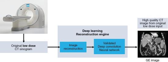
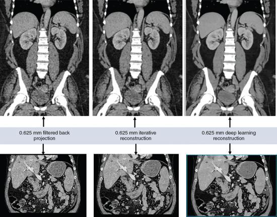
When using the CT scanner with DL reconstruction algorithm in the clinical environment (hospital or clinic), the flow of the reconstruction process using DL algorithms is illustrated in Fig. 6.19. First the CT scanner produces a low-dose CT data set (low-dose sinogram) which goes through the first image reconstruction using either the FBP algorithm or an IR algorithm. Subsequently, these reconstructed images are sent into the deep convolution neural network engine for further processing. The result is a high-quality CT image created from the original low-dose input CT data set. A visual comparison of images reconstructed with the FBP, IR, and DL reconstruction algorithms is shown in Fig. 6.20.
Review questions
Answer the following questions to check your understanding of the materials studied.
- 1. Which of the following is not a key feature of the FBP algorithm-measured projection data (raw data)?
- 2. Which of the following occurs as the last step before the image is created using the FBP algorithm?
- 3. The following are assumptions of the FBP algorithm except:
- 4. The most recent method to reduce noise in low-dose CT imaging is to:
- 5. The following refers to IR algorithms currently available from CT manufacturers:
- 6. With IR algorithms without modeling:
- 7. Which of the following is not an essential step in an IR algorithm without modeling?
- 8. An IR algorithm that models the x-ray tube, image voxels and detectors, etc. is referred to as the:
- 9. Compared to the FBP algorithm, IR algorithms result in all of the following except:
- 10. Performance evaluation studies have compared IR algorithms with the FBP algorithm on all of the following characteristics except:
References
Akagi M, Nakamura Y, Higaki T., et al. Deep learning reconstruction improves image quality of abdominal ultra-high-resolution CT European Radiology 2019;29: 4526-4527 doi:10.1007/s00330-019-06249-x.
Bartak N.A. Image quality assessment of abdominal CT by use of new deep learning image reconstruction: initial experience American Journal of Roentgenology 2020;215: 50-57.
Beister D, Kolditz D. & Kalender W.A. Iterative reconstruction methods in X-ray CT Physica Medica 2012;28: 94-108.
Boedeker K. AiCE deep learning reconstruction. Visions Magazine Canon Medical Systems 2019;2: 28-31.
Brenner D.J. & Hall E.J. Computed tomography: An increasing source of radiation exposure New England Journal of Medicine 2007;357: 2277-2284.
Chartrand G, Cheng P.M, Vorontsov E., et al. Deep learning: A primer for radiologists Radiographics 2017;37: 2113-2131.
Chen H, Zhang Y, Kalra M.K., et al. Low-dose CT with a residual encoder–decoder convolutional neural network IEEE Transactions on Medical Imaging 2017;36: 2524-2535.
Chollet F. Deep learning with python 2018; Manning Publications Shelter Island NY.
den Harder A.M, Willemink M.J, Budde R.P.J, Schilham A.M.R, Leiner T. & de Jong P.A. Hybrid and model-based iterative reconstruction techniques for pediatric CT American Journal of Roentgenology 2015;204: 645-653.
Do S, Song K.D. & Chung J.W. Basics of deep learning: A radiologist’s guide to understanding published radiology articles on deep learning Korean Journal of Radiology 1, 2020;21: 33-41.
Ehman E.C, Yu L, Manduca A., et al. Methods for clinical evaluation of noise reduction techniques in abdominopelvic CT Radiographics 2014;34: 849-862.
Erickson B.J, Korfiatis P, Akkus Z. & Kline T.L. Machine learning for medical imaging Radiographics 2017;37: 505-515.
Gordic S, Desbiolles L, Stolzmann P., et al. Advanced modelled iterative reconstruction for abdominal CT: Qualitative and quantitative evaluation Clinical Radiology 12, 2014;69: e497-e504.
Greffier J, Hamard A, Pereira F., et al. Image quality and dose reduction opportunity of deep learning image reconstruction algorithm for CT: A phantom study European Radiology 2020;30: 3951-3959 https://doi.org/10.1007/s00330-020-06724-w.
Higaki T, Nakamura Y, Zhou J., et al. Deep learning reconstruction at CT: Phantom study of the image characteristics Academic Radiology 1, 2020;27: 82-87 doi:10.1016/j.acra.2019.09.008.
Hounsfield G.N. Computerized transverse axial scanning (tomography), Part 1: Description of the system British Journal of Radiology 1973;46: 1016-1022.
Hsieh J. Adaptive statistical iterative reconstruction 2008; Whitepaper GE Healthcare.
Hsieh J, Nett B, Yu Z, Sauer K. & Thibault J.B. Recent advances in CT image reconstruction Current Radiology Reports 2013;1: 39-51 doi:10.1007/s40134-012-0003-7.
Hsieh J, Liu E, Nett B, Tang J, Thibault J.B. & Sahney S. A new era of image reconstruction: TrueFidelity Technical White Paper on deep learning image reconstruction 2019; General Electric Company USA.
Irwan R., et al. AIDR 3D—reduces dose and simultaneously improves image quality 2011; Europe BV Whitepaper, Toshiba Medical Systems Europe BV.
Jensen C.T, Liu X, Tamm E.P., et al. Deep convolutional framelet denoising for low-dose CT via wavelet residual network IEEE Transactions on Medical Imaging 2018;37: 1358-1369.
Kim J.H, Yoon H.J, Lee E, Kim I, Ki Y. & Bak S.H. Validation of deep-learning image reconstruction for low-dose chest computed tomography scan: Emphasis on image quality and noise Korean Journal of Radiology 2021;22: 131-138 kjronline.org. https://doi.org/10.3348/kjr.2020.0116.
Lee J.G, Jun S, Cho Y.W., et al. Deep learning in medical imaging: General overview Korean Journal of Radiology 4, 2017;18: 570-584.
Lenfant M, Chevallier O, Comby P.O., et al. Deep learning versus iterative reconstruction for CT pulmonary angiography in the emergency setting: Improved image quality and reduced radiation dose Diagnostics 8, 2020;10: 558.
Nakamura Y, Higaki T, Tatsugami F., et al. Possibility of deep learning in medical imaging focusing improvement of computed tomography image quality Journal of Computer Assisted Tomography 2020;44: 161-167 doi:10.1097/RCT.0000000000000928.
Patino M, Fuentes J.M, Singh S, Hahn P.F. & Sahani D.V. Iterative reconstruction techniques in abdominopelvic CT: Technical concepts and clinical implementation American Journal of Roentgenology 1, 2015;205: W19-W31.
Pearce M.S, Salotti J.A, Little M.P., et al. Radiation exposure from CT scans in childhood and subsequent risk of leukemia and brain tumors: A retrospective cohort study Lancet 9840, 2012;380: 499-505.
Qiu D. & Seeram E. Does iterative reconstruction improve image quality and reduce dose in computed tomography? Radiology - Open Journal 2, 2016;1: 42-54.
Seeram E. CT dose optimization Radiologic Technology 6, 2014;85: 655-675.
Seeram E. CT at a glance 2018; Wiley and Sons Ltd Oxford, UK.
Shan H, Zhang Y, Yang Q., et al. 3D convolutional encoder–decoder network for low-dose CT via transfer learning from a 2D trained network IEEE Transactions on Medical Imaging 2018;37: 1522-1534.
Shan H, Padole A, Homavounieh F., et al. Competitive performance of a modularized deep neural network compared to commercial algorithms for low-dose CT image reconstruction Nature Machine Intelligence 2019;1: 269-276 doi.org/10.1038/s42256-019-0057-9.
Shukla, P, & Iriondo, R (2020). Main types of neural networks and its applications – tutorial. Retrieved from https://medium.com/towards-artificial-intelligence/main-types-of-neural-networks-and-its-applications-tutorial-734480d7ec8e. Accessed October 2020.
Shin Y.J, Chang W, Ye J.C., et al. Low-dose abdominal CT using a deep learning-based denoising algorithm: A comparison with CT reconstructed with filtered back projection or iterative reconstruction algorithm Korean Journal of Radiology 3, 2020;21: 356-364.
Smith K. Iterative reconstruction in computed tomography Imaging and Therapy Practice 2013; 15-17.
Suzuki K. Overview of deep learning in medical imaging Radiological Physics and Technology 2017;10: 257-273.
Thibault J.B. Veo CT model-based iterative reconstruction 2010; GE Healthcare Whitepaper.
Toshiba Medical Systems (2015). AIDR 3D. Retrieved from http://www.toshiba-medical.co.jp/tmd/english/products/dose/aidr3d/index.html. Accessed March 2015.
Zeng G.L. & Zamyatin A. A filtered back projection algorithm with ray-by-ray noise weighting Medical Physics 3, 2013;40: 031113.