10: Radiation dose in computed tomography
Learning objectives
On completion of this chapter, you should be able to:
- 1. state two reasons why the dose in CT is of importance to the CT technologist.
- 2. explain what is meant by exposure, absorbed dose, and effective dose.
- 3. explain what is meant by stochastic effects and deterministic effects of radiation exposure, and provide examples of each class of bioeffects.
- 4. describe the characteristics of the CT beam geometry that affect the dose distribution in a patient.
- 5. state the function that describes an arbitrarily shaped dose intensity along the patient axis.
- 6. state several methods for measuring the dose in CT.
- 7. describe what is meant by the CTDI, MSAD, and DLP.
- 8. describe the characteristics of CT scanner dosimetry phantoms.
- 9. describe briefly the basic steps of the CT dose measurement procedure.
- 10. outline the factors affecting dose in CT and explain various dose reduction methods.
- 11. describe the basic principles of automatic tube current modulation.
- 12. state what is meant by iterative reconstruction (IR) and deep learning reconstruction (DLR) algorithms.
- 13. describe the effects of IR and DLR algorithms on dose reduction.
- 14. identify two major categories of biological effects of radiation exposure.
- 15. explain what is meant by radiation protection philosophy.
- 16. outline major optimization strategies.
- 17. define the term diagnostic reference level (DRL).
- 18. explain briefly how DRLs are established and how the values are set.
CT use and dose trends
Since its introduction in the early 1970s, computed tomography (CT) has played a significant role in the detection and management of human diseases in medicine (Rubin, 2014). The technical evolution of CT has been dynamic, ranging from the first-generation, single-slice “stop-and-go” technique to multislice volume CT scanning. Volume CT scanners continue at a rapid rate, from 16- to 64-slice systems, including the 320-slice CT scanner. These developments have created a wide variety of clinical applications such as CT colonography, CT perfusion, CT angiography, cardiac CT imaging (Hedgire et al., 2017; Kwan et al., 2021; Litmanovich et al., 2014; Rubin, 2014), CT screening, and the increasing use of three-dimensional (3D) visualization techniques (Blum et al., 2020) including recent techniques such as cinematic rendering (Eid et al., 2017) and global illumination (Canon Medical Systems, 2019) to enhance diagnosis.
Furthermore, there has been an increase in CT use in the United States and elsewhere (Feng et al, 2013; Smith-Bindman et al., 2019). Coupled with the expanding use of CT in medicine, one other major concern receiving increasing attention in the literature relates to the potential for high radiation doses to be delivered by CT scanners (Gottumukkala et al., 2019: Hedgire et al, 2017; Papadakis, 2016; Parakh et al., 2016).
All individuals working in CT, such as radiologists, technologists, medical physicists, physicians, and manufacturers, should ask three questions that have been the central focus of the topic of CT dose: Why are the doses in CT so high? What is the dose to the patient at my institution? What can be done to reduce the high exposures in CT to protect both patients and personnel?
There are several reasons why these questions are important; however, the most important reason for understanding radiation dose in CT relates to radiation risks. Numerous studies have shown, however, that patient doses from CT examinations are high relative to other radiography examinations (Berrington et al., 2009; Brenner & Hall, 2007; Van der Molen, 2013) and that CT doses typically range from 5 to 50 mGy to each organ within the image field (Mathews et al., 2013). As of 2011, CT contributed the highest collective amount of medical radiation exposure in the United States compared with any other medical imaging modality (Hricak et al., 2011). The relatively high doses related to CT examinations, particularly for pediatric patients, have called attention to the risks of cancer associated with CT scanning (Amis, 2011; Brenner & Hall, 2007; Hendee & O’Connor, 2013; Mathews et al., 2013)
The dose for a CT examination may have to be estimated to make decisions regarding the benefits versus the risks of the procedure. CT manufacturers are now required by law to provide a dose table that shows the doses delivered to patients from their CT scanners.
The purpose of this chapter is to outline the fundamental concepts of radiation dose in CT. In particular, topics such as radiation quantities and their units; factors affecting dose in CT; and CT dosimetry, including dose descriptors, phantoms and measurement concepts, automatic exposure control (AEC) in CT, dose reduction technology, dose optimization strategies, and radiation protection considerations are described.
Radiation quantities and their units
The literature on radiation dose in CT reports the dose in CT using various radiation quantities (exposure, absorbed dose, and effective dose) and their associated units: Roentgens, rads, and rems (old units), respectively, or coulombs per kilogram, Grays, and Sieverts (International System of units = SI units), respectively (Bushberg et al., 2012; Bushong, 2017; Seeram, 2020) For this reason, a brief review of these quantities and units is necessary. The radiation quantities of relevance to this chapter are exposure, absorbed dose, and effective dose. For a more comprehensive description of these quantities and units, the reader may refer to Seeram and Brennan (2017).
Exposure
The radiation quantity, exposure, refers to the concentration of radiation at a particular point on the patient. Exposure is easy to measure with an ionization chamber positioned at the point of measurement. Radiation falling on the chamber ionizes the air in the chamber to produce ion pairs (charges). Exposure is a measure of the amount of ionization produced in a specific mass of air by x rays or gamma radiation. The ionization indicates the amount of radiation to which a patient is exposed.
The unit of exposure is the Roentgen (R), the conventional unit, or the coulomb per kilogram (C/kg), the SI unit. One Roentgen produces 2.58 × 10⁻⁴ C/kg of air at standard temperature and pressure. Exposure is reported in the literature in milliroentgens (mR), a much smaller unit (1 R = 1000 mR) or in microcoulombs/kilogram (μC/kg) where 1 R = 258 μC/kg.
Absorbed dose
The absorbed dose, or radiation dose as it is popularly referred to, is the amount of energy absorbed per unit mass of material (patient). Any risk associated with radiation is related to the amount of energy absorbed, and this quantity is particularly important in radiation protection.
The old unit of absorbed dose is the rad (r), which is equal to an energy absorption of 100 erg/g of absorber. The SI unit of absorbed dose is the Gray (Gy), so named in honor of Louis Harold Gray, a British radiobiologist who devised ways to measure the absorbed dose. One Gray is equal to 1 joule per kilogram (J/kg) or 1 r is equal to 0.01 Gy or 100 r is equal to 1 Gy. Relevant submultiples of the Gray are 1 centigray (cGy), which equals 1 r and 1 milligray (mGy), which equals 100 millirads (mrads). For the sake of simplicity, 1 r is approximately equal to 0.01 Gy.
Effective dose
The quantity effective dose, E, previously referred to as the effective dose equivalent, is used to quantify the risk from partial-body exposure to that from an equivalent whole-body dose. The term is used to take into account the type of radiation (because different types of radiation can produce varying degrees of biological damage) and the radiosensitivity of different tissues (because some tissues are more sensitive than others).
As described by McNitt-Gray (2002), E is a “weighted average of organ doses” and can be expressed mathematically as follows:

where DT,R is the absorbed dose to the tissue (T), WT is the tissue-weighting factor, WR is the radiation-weighting factor, and the symbol ∑ is the “sum of.” These factors can be obtained from previously calculated tables (Bushong, 2017).
Although the old unit of effective dose is the rem, the SI unit is the Sievert (Sv), where 1 Sv = 100 rem. The effective dose relates exposure to risk. As noted by Brenner (2006), “relevant organ doses for CT examinations are on the order of 15 mSv or less.” Brenner also notes that “there is good epidemiologic evidence of increased cancer risk for children exposed to acute doses of 10 mSv (or more) and for adults exposed to acute doses of 50 mSv (or more).”
To put this into perspective, emphasized that “the total amount of radiation that a patient receives in any radiographic examination is best quantified by the effective dose, which is related to the risk of carcinogenesis, and with the induction of genetic effects. Effective doses with radiographic imaging are smaller than natural background (3 mSv per year). Effective doses from common fluoroscopic and CT examinations are comparable to natural background and may be much higher with interventional radiology procedures.”
It is interesting to recall that the dose limits for occupationally exposed individuals (radiologists and technologists, for example) are given in mSv. The International Commission on Radiological Protection (ICRP) dose limit for radiation workers is 20 mSv per year. Although the dose limits for radiation workers in the United States is 50 mSv per year, it is 20 mSv per year for workers in Canada (Bushong, 2017).
Radiation bioeffects
One of the reasons technologists and radiologists should have a clear understanding of the dose in CT relates to radiation bioeffects. These effects are classified as stochastic and deterministic. It is not within the scope of this chapter to describe the details of these effects; however, for the sake of relating these effects to dose in CT, a brief review is necessary. For a more detailed account of the risks, the interested reader should refer to the paper by Hendee and O’Connor (2013).
Stochastic effects
Stochastic effects are those effects for which the probability (rather than the severity) of the effect occurring depends on the dose. The probability increases with increasing dose, and there is no threshold dose for these effects. The linear no threshold (LNT) dose–response model is the radiation risk model most favored by radiobiologists in estimating the risk of exposure in radiology (Bushong, 2017). Medical radiation protection standards, guidelines, and recommendations are based on this model.
The LNT dose-response model states that the radiation risk increases as the dose increases and there is no threshold dose. Hendee and O’Connor (2013) stated that the LNT model is more commonly used because it is a simpler and conservative approach, which is more likely to overestimate cancer risk at low doses than to underestimate risk of cancer induction. The authors further stated, however, that because medical imaging doses are so low, there is no evidence that the no-threshold model is effective at estimating cancer induction risk.
Furthermore, even a small dose has the potential to cause a biological effect. There is no risk-free dose. If harm occurs, the damage generally becomes apparent years after exposure; therefore, stochastic effects also are called late effects. Examples of stochastic effects include cancer, leukemia, and hereditary effects. Stochastic effects are considered a risk from exposure to the low levels of radiation used in medical imaging, including CT examinations.
Deterministic effects
Deterministic effects (nonstochastic effects) are those effects for which the severity of the effect (rather than the probability of the effect) increases with increasing dose and for which there is a threshold dose. Below the threshold dose, these effects are not observed. Threshold doses are considered to be relatively high doses that can kill cells and cause degenerative changes in tissues that have been exposed to radiation. Deterministic effects are also referred to as early effects and involve high exposures that are unlikely to occur in medical imaging examinations.
Examples of deterministic effects include skin erythema, epilation, and pericarditis for example. Absorbed doses in CT are substantially lower than threshold doses for the induction of deterministic effects. As patients undergo several examinations, it may be possible to reach the threshold dose for certain deterministic effects.
Patient exposure patterns in radiography and CT
It is clearly apparent that the geometry of the x-ray beam and the way in which the patient is exposed to the beam is different in radiographic imaging and in CT imaging, as shown in Fig. 10.1. In radiography, the x-ray tube is typically above the patient in a fixed position as the examination is conducted, and the shape of the beam is a cone. This shape is sometimes referred to as open-beam geometry. Although the entrance exposure is 100%, it is sometimes used to represent risk; however, this is an overestimation because the dose decreases as it passes through the patient. Such decrease is due to attenuation and the inverse square law. The dose distribution for radiographic imaging is illustrated in Fig. 10.1A.

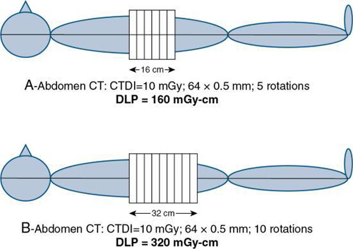
In CT, the exposure pattern is somewhat different from that of radiography because of the geometric aspects of the beam and the scanning procedure. In general, the beam is well collimated to describe a fan-shaped beam that rotates around the patient at least for 360 degrees. The x-ray tube is not fixed as in radiography but assumes several positions during one complete revolution around the patient. In modern multislice CT scanners, the fan-shaped beam has now become a cone-shaped beam (see Chapter 12). The dose distribution pattern is more uniform in CT (Fig. 10.1B) compared with radiography because the x-ray beam is rotating 360 degrees around the patient’s body. Typical dose values for a 16-cm diameter head phantom and a 32-cm diameter body phantom, respectively, are given in Fig. 10.2.

CT scanner x-ray beam geometry
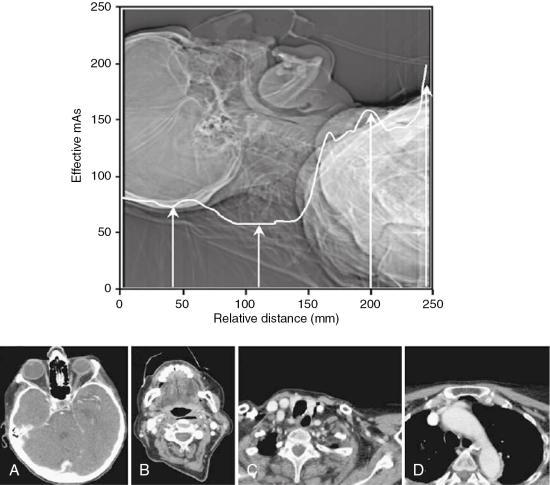
The term beam geometry refers to the size and shape of the x-ray beam emanating from the x-ray tube and passing through the patient to strike a set of detectors that collects radiation attenuation data. The beam geometry and the nature of the scanning process in multislice CT (MSCT) imaging are shown in Fig. 10.3, in which a fan-shaped x-ray beam and an array of detectors rotate 360 degrees around the patient to collect attenuation data. The table moves during the scanning process, and the x-ray tube traces a spiral or helical beam path around the patient.
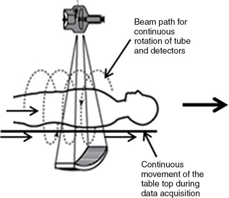
Fig. 10.4A shows the same fan-shaped x-ray beam viewed from the side with the thickness exaggerated for clarity. If the longitudinal (cranial–caudal) axis of the patient is defined as the z-axis, then in theory the intensity of the radiation beam along that axis can be graphed. Ideally the radiation intensity measured along the z-axis would have equal intensity everywhere inside the beam and would have no intensity on either side. Fig. 10.4B shows this ideal rectangular intensity profile of the radiation beam. In reality, the radiation intensity measured along the z-axis has smoother edges and appears as a bell-shaped curve. The dose distribution is almost always wider than the nominal slice width (SW).

The dose distribution is given by the function D(z), which describes an arbitrarily shaped dose intensity along the patient axis. In general, the shape of D(z) varies among CT scanners. D(z) is extremely important to dose in CT because it is the dose distribution measured. The instrumentation and methods used to measure patient dose from a CT scanner is referred to as CT dosimetry, and it is uniquely different compared with the dosimetry of projection radiographic imaging.
CT dosimetry concepts
CT dosimetry is an important concept for CT technologists for several reasons. First, technologists can compare their hospital CT doses with the national average to find out whether their radiation protection efforts are comparable to those of others. Second, technologists can participate effectively in informing both the public and other hospital personnel (physicians and nurses, for example) about the dose in CT. Third, and perhaps more important, CT technologists can assist the medical physicist with not only performing the actual dose measurements (this has been identified as one of the duties of a certified medical physicist by the American College of Radiology) but also being a more integral part of CT acceptance testing and continuing quality control procedures. Finally, a knowledge of CT dosimetry will assist the technologist in conducting dose measurements in cases where there is no medical physicist to perform this task.
The nature of CT dosimetry is complex and challenging because of the continuous technological evolution of CT scanners. Dosimetry involves the measurement of the dose to the patient and is characterized by several metrics. These metrics refer to radiation dose quantities and their associated units.
It is not within the scope of this text to describe how to conduct the actual dose measurements and how to estimate the radiation doses to patients because these are topics within the domain of medical physicists. It is important, however, to highlight several important and essential concepts, including types of dosimeters used to measure CT doses, CT dosimetry phantoms, and dose descriptors specific to CT.
Types of dosimeters
In the past, several types of dosimeters were used to measure the dose in CT. These include film dosimeters, thermoluminescent dosimeters (TLDs), and specially designed ionization chambers. In 1981, the Bureau of Radiological Health (BRH), now the Center for Devices and Radiological Health (CDRH), introduced what could be noted as a significant step toward CT dose measurement. The method suggested by the CDRH uses a pencil ionization chamber. Solid-state metal oxide semiconductor field effect transistors (MOSFET) are now used in CT dosimetry studies because they are more sensitive than TLDs, they provide an instant readout, and they can be reused immediately. For further details on the methodology for the evaluation of radiation dose in x-ray CT, the interested reader may refer to the American Association of Physicists in Medicine (AAPM) Report No 111 (2010).
Ionization chamber
An ionization chamber is an instrument used to accurately quantify radiation exposure. The ionization chamber shown in Fig. 10.5 consists of a small air-filled container with thin walls that allow radiation to pass through easily. As the high-energy photons (x rays) collide with air molecules enclosed within the ionization chamber, some of the molecules are “ionized” (i.e., one or more electrons are knocked from some molecules). These free electrons can be collected on a conducting wire or plate and measured as electric charge. The amount of collected charge is proportional to the amount of ionization, which is proportional to the amount of radiation that passes through the chamber. The charge is removed from the ionization chamber and measured with a very sensitive instrument known as an electrometer. The total electric charge generated by an x-ray beam is represented by Q and measured in coulombs (1 coulomb = 6.24 × 10¹⁸ electrons).

Phantoms for CT dose measurement
To standardize the measurement of the dose and provide a clinically realistic geometry, the BRH researchers suggested that the ionization chamber be placed in one of two cylindrical phantoms during the radiation measurement. The smaller phantom simulates a patient’s head and the larger phantom simulates a “body” or torso (Fig. 10.6). Both phantoms are 15 cm in length. The diameter of the “head” phantom is 16 cm, and the diameter of the “body” phantom is 32 cm. Both phantoms are solid acrylic with holes drilled through the phantom at specified locations to accommodate the pencil ionization chamber (Fig. 10.7). Acrylic plugs are placed in the holes unoccupied by the ionization chamber. Fig. 10.8 shows a pencil ionization chamber about to be inserted into a CT scanner dosimetry phantom. The holes that are not used for the ionization chamber are filled with acrylic plugs. Careful examination of the plug reveals a small hole that can be seen through its diameter. This hole is centered end to end in the plug and is visible in the CT image of the dosimetry phantom if the x-ray beam is centered on the phantom and passes through the hole. The appearance of the hole in the image verifies that the x-ray beam is striking the center of the phantom.


The procedure for measurement is to place the ionization chamber in one of the phantom holes, take a scan, and record the amount of charge emitted from the chamber. Then the chamber is moved to the next hole, the plug is placed in the original chamber hole, and the procedure is repeated. Moving the chamber to another hole (e.g., from the anterior to the posterior) allows the dose to be determined at a variety of locations within the phantom. Generally, the dose varies among locations, even when the same technique is used. For example, the dose at the anterior location of the phantom differs from the dose at the posterior location, which differs from the dose on the patient’s right side, and so on. It is usually prudent to measure the dose at several locations for a given technique.
Display of CT dose metrics on the scanner
In general, there are four CT dose metrics (to be described subsequently) commonly used in CT, and are typically shown on the dose report that displays on the CT scanner console. These include the CT dose index (CTDI), the dose-length product (DLP), and the size-specific dose estimate (SSDE). The SSDE depends not only on the radiation output from the CT scanner but also the size of the patient. The fourth dose metric of importance in CT, and in any imaging modality using ionizing radiation, is the effective dose.
The International System of Units quantity for the CTDI and the DLP is expressed in milligrays (mGys); it is expressed in millisieverts (mSv) for the effective dose. The effective dose relates the radiation exposure to risk and is considered the best method available to estimate stochastic radiation risk (Wolbarst et al., 2013). Still, effective dose is an estimate only, based on weighting factors applied to the body’s tissue or the organ being irradiated (Hermann et al., 2014).
CT dose metrics and calculation
The earlier dose studies reported CT doses by using various terms to describe the absorbed dose in a CT examination. These included single-scan peak dose, multiple-scan peak dose, dose profile, and others such as multiple-scan average dose (MSAD). These results led the CDRH to introduce and recommend the use of CTDI and MSAD in the Federal Performance Standard as the dose descriptors specific to CT. For example, because the early CT examinations consist of a series of stop-and-go scans (slices), the MSAD was the dose descriptor for use in a clinical situation at that time. The MSAD concept will be highlighted for historical reasons only.
Multiple-scan average dose
The MSAD was the first CT dose descriptor to be identified (Cody & McNitt-Gray, 2006; McNitt-Gray, 2002). To use the MSAD, a series of CT scans is performed on a patient (Fig. 10.9). Between each scan, the patient is moved a bed index (BI) distance. Each slice delivers the characteristic bell-shaped dose represented by the curves at the top of Fig. 10.9. If the doses from all scans are summed, the resulting total patient dose resembles the oscillating curve at the bottom of Fig. 10.9. In the regions where the bell curves overlap, the resultant dose is higher than that from just one scan. If the total dose distribution curve is known (bottom curve), the MSAD (dotted straight line) can be calculated by mathematically sampling the peaks and valleys of the multiple scan dose curve. This can be written as follows:


where SW is slice width in millimeters and BI is bed index or slice spacing.
Computed tomography dose index
The CTDI was the next CT dose descriptor after the MSAD. It was developed by the US Food and Drug Administration (FDA) and was therefore labeled CTDIFDA (Boone, 2007). CTDIFDA has evolved to its present form with several notable changes. These are highlighted in this subsection.
The CTDIFDA is defined as follows:
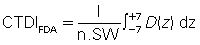
where n is the number of distinct planes of data collected during one revolution, SW is the nominal slice width in millimeters, D(z) is the dose distribution, and z is the dimension along the patient’s axis. For axial (non-spiral/helical) CT scanners and spiral/helical CT scanners with a single row of detectors, n = 1. For MSCT scanners, n is the number of active detector rows (n = 16) during the scan.
The CTDIFDA represents the mean absorbed dose in the scanned object volume; therefore, the unit of the CTDI is Gy with relevant submultiples such as cGy and mGy.
This equation is not as complicated as it appears. The integral sign (∫) merely instructs the user to determine the area under a single curve D(z). Fig. 10.10 demonstrates the value of this integral by shading the area under a typical dose distribution curve. If this area is divided by the number of slices times the slice width [(n)(SW)], the result is the CTDIFDA.

This definition, which was accepted by the International Electrotechnical Commission (IEC, 2001), is good for essentially all shapes of dose distribution curves D(z) that are emitted by CT scanners. Note that increasing the area under the curve can increase the CTDIFDA. The area can be increased by either increasing the intensity of radiation, which raises the height of the curve, or by widening the curve, usually by opening the x-ray collimators near the x-ray tube. Either case increases the CTDIFDA and ultimately increases the radiation dose to the patient.
For axial CT scanners, as the slice spacing increases, there is a greater likelihood that relevant tissue will be “missed” (it falls between the slices) in the scan sequence, thus limiting the amount that the BI can be increased. Conversely, when the BI is made smaller, the slices become closer together, more overlap of adjacent dose distributions occurs, and the average dose increases. When the SW equals the BI, the MSAD is numerically equal to the CTDIFDA.
The CTDIFDA has evolved from its initial stage of measurement for 14 contiguous slices where the integration would be from –7 to +7. The fixed length of the pencil ionization chamber “meant that only 14 sections of 7-mm thickness could be measured with that chamber alone. To measure CTDIFDA for thinner sections, sometimes lead sleeves were used to cover the part of the chamber that exceeded 14 section widths” (Cody & McNitt-Gray, 2006; McNitt-Gray, 2002).
This shortcoming was solved by introducing another dose index, the CTDI100, which “relaxed the constraint on 14 sections and allowed calculation of the index for 100 mm along the length of the entire pencil ionization chamber, regardless of the nominal slice width being used” (McNitt-Gray, 2002). The index is given by the equation:
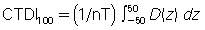
where nT is the nominal collimated slice thickness.
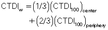
The next major change in the CT dose descriptor is the introduction of the weighted CTDI (CTDIW) to account for the average dose in the x-y axis of the patient instead of the z-axis. This can be done using a phantom where the pencil ionization chamber is positioned in the center (CTDIcenter) and at the periphery (CTDIperiphery) of the phantom (see Fig. 10.7). In this case the following algebraic expression can be used to calculate the CTDIW (as provided by Cody & McNitt-Gray [2006] and McNitt-Gray [2002]):
To consider the dose in the z-axis, yet another dose descriptor was developed. This is the CTDIvolume, which can be calculated with the following relationship for spiral/helical CT imaging:

It is important to note that the term pitch has been defined by the IEC as a ratio of the distance the table travels per revolution (in millimeters) to the total nominal beam collimation (in millimeters). For a pitch of 1, the CTDIvolume is equal to the CTDIW; for a pitch of 1.5, the CTDIvolume is equal to CTDIW/1.5.
Dose length product
As mentioned earlier, the DLP is yet another dose descriptor used in CT dose studies and reported in the literature and on CT scanners. Although the CTDIvolume provides a measurement of the exposure per slice of tissue, the DLP provides a measurement of the total amount of exposure for a series of scans. The DLP can be calculated if the length of the irradiated volume (scan length) and the CTDIvolume are known by using the following relationship:

It is important to note that, although the CTDIvolume is not dependent on the scan length, the DLP is directionally proportional to the scan length (Fig. 10.11). DLP is expressed in mGy-cm.
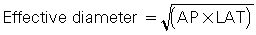
Size-specific dose estimate
Another CT dose metric introduced by the AAPM in 2011 (Tsujiguchi et al., 2018; Waszczuk et al., 2015) to account for patient size is the size-specific dose estimate (SSDE) as the CTDIvolume and DLP do not address smaller pediatric patients. The SSDE takes into consideration the size of the patient to obtain the CTDIvolume. The size dimensions of the anteroposterior (AP) and lateral (LAT) measurements of the patient are used to calculate the effective diameter which “represents the diameter of the circle whose area is the same as that of the patient’s cross-section” (Waszczuk et al., 2015). Furthermore, these dimensions can be “measured using electronic calipers on the axial scans at the center of the scanned volume along the z-axis (cranio-caudal)” (Waszczuk et al., 2015). The effective diameter can be obtained using the following relationship:
The SSDE is obtained using the following equation:

where
a = 3.704369; and b = 0.03671937. A study by Waszczuk et al., (2015) showed that the SSDE (mGy) mean ± SD for patient sizes of less than 30 cm, between 30 and 35 cm, and greater that 35 cm in routine dose CT were 6 ± 3; 24 ± 5; and 34 ± 2, respectively.
In a study examining the usefulness of a size-specific dose estimate in pediatric CT examination, Tsujiguchi et al. (2018) found that “when estimating the organ dose and effective dose for pediatric patients and the standard and thin body type patients, the SSDE-corrected value is less likely to underestimate the exposure dose than the conventional method using CTDIvolume and DLP, making SSDE a very effective method.”
Effective dose
The next stage in this area of patient dose assessment is to address the risk of a CT examination. This requires the use of the effective dose. Effective dose is used in radiation protection to relate exposure to risk, and it takes into account that different tissues have different radiosensitivities and the absorbed dose to specific organs. For example, the gonads are more radiosensitive than the brain (Bushong, 2017). Because only parts of the body (rather than the entire body) are exposed in medical diagnostic imaging, risk of stochastic radiation response is proportional to the effective dose rather than to the tissue dose. The effective dose is expressed by the following:
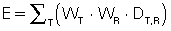
where WT = tissue weighting factor, WR = radiation weighting factor, and DT,R = average absorbed dose to tissue T. The tissue and radiation weighting factors are available from tables provided by the ICRP and the NCRP.
The SI unit for E is the Sievert; whereas the old unit is the rem.

For simplicity, the effective dose is obtained by multiplying the DLP by constants referred to as k values, which have been previously established. For example, the k value (mSv/mGy-cm) for a CT scan of the head is 0.0021; the k value is 0.015 for a CT scan of the pelvis (McNitt-Gray, 2002). Knowing these k values enables calculation of the effective dose as follows:

The effective dose allows for a comparison of the dose received from CT scanning with the dose received from natural background radiation. For example, Bushong (2017) noted that while the annual effective dose from natural background radiation is reported to be 3 mSv, it is 1.5 mSv for CT and 3 mSv for medical imaging (CT scanning, radiography, and interventional, nuclear medicine).
Measuring the CT dose index
It is not within the scope of this book to describe the details of how to measure the CTDI because this is usually, a task for the medical physicist. However, the following steps are noteworthy, using the phantoms and pencil ionization chamber described earlier:
- 1. The pencil ionization chamber is placed into one of the holes in the phantom, perpendicular to the fan of the radiation beam (i.e., the chamber is placed parallel to the longitudinal axis of the patient; see Fig. 10.5), and the other holes are plugged with acrylic plugs.
- 2. An exposure is made for a single scan, and the chamber measures the exposure (not dose). The chamber intercepts the entire narrow width of the x-ray beam. The x-ray beam must be positioned in the center of the chamber.
- 3. The chamber converts the x rays into charge. This charge represents the integral in Equation 10.2.
- 4. The ionization chamber receives radiation from all parts of the dose distribution D(z) because of its length. The total charge from the ionization chamber is proportional to the integral in the CTDI definition. Mathematically, this is expressed as follows:
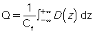
where Q is the total charge collected during a single scan and Cf is the calibration factor of the ionization chamber. Because the ionization chamber measures exposure and not the dose, a conversion factor (the f factor) must be included in Cf, which converts exposure (in Roentgens, R) to dose (cGy; recall that 1 cGy = 1 rad). The value of the f factor at CT scanner x-ray energies is approximately 0.94 cGy/R.
An interesting point to note about the CTDI is that the integration range is restricted to single-slice CT scanners collimated to beam widths of 10 mm and less (Boone, 2007) and to 100 mm for the CTDI100. For example, the nominal beam width for the 256-slice CT scanner is 128 mm; therefore, the integration range has increased to 300 mm for an accurate measurement of the dose from this CT scanner.
Factors affecting the dose in CT
Several factors affect the dose in CT. These fall into two categories, namely, those that have a direct effect on the dose and those that have an indirect effect on the dose (Cody & McNitt-Gray, 2006; Kalra et al., 2004; McNitt-Gray, 2002). Although the direct factors are those factors that increase or decrease the dose to the patient and are under the direct control of the technologist, the indirect factors are those that “have a direct influence on image quality, but no direct effect on radiation dose; for example, the reconstruction filter” (McNitt-Gray, 2002). It is beyond the scope of this chapter to describe all of these factors; therefore, only the factors that have a direct effect on the dose to the patient, and those where the technologist has some degree of control, are reviewed. These include the exposure technique factors, x-ray beam collimation, pitch, patient centering, number of detectors, and over-ranging, also referred to as z-overscanning, and iterative and deep learning (subset of machine learning, a subset of artificial intelligence) reconstruction.
Exposure technique factors
Exposure technique factors are characterized by the tube potential defined by the kilovoltage; tube current, defined by the milliamperage; and the exposure time in seconds. The product of the milliamperage and the exposure time is the milliamperage-seconds (mAs). The technologist can select these factors manually or they can be selected by using automatic exposure control (AEC), which uses a technique known as automatic tube current modulation and is described later in the chapter.
Constant milliamperage-seconds
The term constant mAs refers to the selection of milliamperage and time (in seconds) separately or mAs on some scanners before the scan begins, keeping all other technical factors constant. The mAs determines the quantity of photons (dose) incident on the patient for the duration of the exposure. The dose is directly proportional to the mAs, and if the mAs is doubled, the dose will be doubled.
Effective milliamperage-seconds
The effective mAs is a term used for MSCT scanners that denotes the mAs per slice. This is given by the following relationship:

This expression simply implies that, to keep the effective mAs constant, as the pitch increases, the true mAs must be increased as well. For example, increasing the pitch from, say, 1 to 2, increases the mAs per rotation from 100 to 200 while the relative CTDIvolume remains the same (Lewis, 2005).
Peak kilovoltage
The peak kilovoltage (kVp) determines the penetrating power of the photons coming from the x-ray tube. Higher kVp means that the photons have higher energies and can penetrate thicker objects compared with lower kVp x-ray beams. In CT generally, for adult imaging, high kVp techniques are used, such as 120 kVp. The radiation dose is proportional to the square of the kVp (Bushberg et al., 2012). This means that the quantity of photons increases by the square of the kVp. A 72-kVp technique will have fewer photons than a kVp of 82, all factors held constant.
Collimation (z-axis geometric efficiency)
In CT, the collimation is used to define the beam width for the examination. Collimation schemes are different between single-slice (single detector row along the z-axis) and MSCT scanners. The collimation reflects the efficient use of the x-ray beam at the detector, as shown in Fig. 10.12. The shaded portion represents the penumbra caused by the finite size of the x-ray tube focal spot. It is clearly apparent that on a single-slice CT scanner, the entire beam width plus the penumbra fall on the detectors. The penumbra, however, is not used to produce the image, but it does affect the patient dose.

On MSCT scanners, the beam width, including the penumbra, would fall on a finite set of detectors depending on the scanner, but the penumbra would not be used to produce the image (because the intensity of the beam at the penumbra regions is less than the intensity at the center of the beam). To address this problem, the beam width (collimation) is increased so that the penumbra extends beyond the active detectors that will receive the central beam intensity (Lewis, 2005). The ratio of the area under the z-axis dose profile falling on the active detectors to the area under the total z-axis dose profile is referred to as the z-axis geometric efficiency (IEC, 2001).
Cody and McNitt-Gray (2006) showed that for a 32-cm diameter phantom, as beam widths increase from 18.0 mm, 19.2 mm, 24.0 mm, and 28.8 mm, the CTDIw (mGy) changes from 15.7 mGy, 16.8 mGy, 15.0 mGy, and 13.9 mGy, respectively (all other technical factors held constant). Additionally, Lewis (2005) indicated that “scanners that acquire a greater number of simultaneous slices have an advantage in terms of z-axis geometric efficiency. This is because for narrow slice widths a wider total collimation can be used. On multislice scanners z-axis geometric efficiencies are generally in the range of 80–98% for collimators of 10 mm and above, and about 55–75% for collimators of around 5 mm. For collimators around 1-2 mm z-axis geometric efficiencies are as low as 25% on some systems, although in dual slice mode, they can be much higher. Therefore, the reduced geometric efficiency of multislice scanners, for wider collimators most commonly used, leads to dose increases around 10% when compared with single slice systems. However, very narrow collimations can result in a tripling, or more, in dose”.
Pitch
The term pitch is one common to spiral/helical CT scanners, sometimes called spiral pitch or helical pitch, depending on the manufacturer of the scanner. As defined by the IEC, pitch is a ratio of the distance the table travels per rotation to the total collimated x-ray beam width. The relationship between the absorbed dose and pitch is as follows:

Therefore, if the pitch increases by 2, the dose will be reduced to one half. It is important, however, to note that this relationship only holds true when the pitch changes and all other factors remain constant. For constant mAs (100 mAs per rotation), if the pitch changes from 1 to 2, the relative CTDIvolume decreases from 1.0 to 0.5 mGy (Lewis, 2005).
Number of detectors
In a study comparing the dose from CT scanners, Moore et al. (2006) demonstrated that the measured radiation dose is inversely proportional to the number of detector rows. They showed that there is a trend that as the number of detector rows increases from 4 to 8 to 16 detector rows, the dose decreases with both standard and near identical technique.
Over-ranging (z-overscanning)
In spiral/helical CT scanning, it is important to realize that to image the planned length of tissue required for the examination and of interest to the radiologist, additional rotations before and after the planned length are essential for the image reconstruction process. This is referred to as over-ranging or z-overscanning (Tzedakis et al., 2007; Van der Molen and Geleijns, 2007), of which the components and definitions developed by Van der Molen and Geleijns (2007) are clearly illustrated in Fig. 10.13. It is clear that there are two definitions of over-ranging:

Over-ranging increases the dose to the patient, which is validated in studies conducted by Tzedakis et al. (2007) on pediatric patients and by Van der Molen and Geleijns (2007). For example, Tzedakis et al. (2007) concluded that “in all cases normalized effective dose values were found to increase with increasing z-overscanning. The percentage differences in normalized data between axial and helical scans may reach 43%, 70%, 36%, and 26% for head-neck, chest, abdomen-pelvis, and trunk studies, respectively.” Van der Molen and Geleijns (2007), for example, concluded that “overranging is reconstruction algorithm specific, and its length generally increases with collimation and pitch, while the effect of section width is variable. Over-ranging may lead to substantial but unnoticed exposure to radiosensitive organs.”
Patient centering
Another factor affecting the dose to the patient under the control of the technologist is that of patient centering. The patient must be centered in the gantry isocenter for accurate imaging of the anatomy. Inaccurate patient centering (miscentering or off-centering), as shown in Fig. 10.14, degrades the image quality and increases the dose to the patient, especially with the use of AEC in CT (Barreto et al., 2019; Euler et al., 2019; Isa et al., 2018; Saltybaeva et al., 2017). Additionally, the use of bowtie filters in CT scanners is intended to serve basically two purposes: to shape the beam intensity within the scan field of view (SFOV) and to produce a more uniform beam at the detectors (see Chapter 4). The x-ray beam is filtered; therefore, the bowtie filter actually plays a small role in reducing the dose to the patient because the low-energy photons are removed and thus the beam becomes harder, that is, the mean energy of the beam increases. Improper centering of the patient in the gantry isocenter as shown in Fig. 10.14 can lead to an increase in surface dose as well as the peripheral dose to the patient (Barreto et al., 2019; Euler et al., 2019; Isa et al., 2018; Saltybaeva et al., 2017). Furthermore, Kaasalainen et al., (2014) showed that miscentering was more pronounced in smaller pediatric patients, in terms of dose and image noise.

These findings are positive proof that technologists should always center the patient accurately in the gantry isocenter to avoid image noise problems and reduce the dose to the patient.
Automatic tube current modulation
AEC is now commonplace on CT scanners. AEC uses a technique referred to as automatic tube current modulation (ATCM) to optimize the dose to the patient while maintaining constant image quality, regardless of the size of the patient, in the z-axis and the attenuation changes in the x-y axis (McNitt-Gray, 2011; Supanich, 2013). ATCM has been hailed as “the most important technique for maintaining constant image quality while optimizing radiation dose” (Li et al., 2007), and especially in pediatric CT (Papadakis & Damilakis, 2019). For this reason, ATCM is described in detail in the next section.
Automatic tube current modulation
ATCM is a technical development in CT based on the fundamental principles of AEC (Supanich, 2013). AEC is not a new concept for radiologic technologists, for it is used extensively in radiography and fluoroscopy. The purpose of AEC in radiography, for example, is to provide a level of image quality (expressed as optical density for film-based radiography) in which there is consistent optical density for any examination (e.g., chest x ray) regardless of the thickness (small, medium, and large) of the patient. This level of image quality (optical density) is controlled by varying the duration of the exposure on the basis of the size of patient being imaged. For example, although the duration of the exposure will be shorter for smaller patients, it will be longer for larger patients, and therefore images of the same body parts on these patients will all have a consistent level of optical density.
Problem with setting manual milliamperage techniques
In CT, the exposure technique factors (mAs and kVp) do not have a direct effect on the image density and contrast, respectively (as they do in film-based radiography), because CT is a digital-imaging modality. The dose to the patient is directly proportional to the mA, and in the past, CT technologists selected the mA values for patients manually. Lewis (2005) explained one of the problems with setting the mA values manually. She noted:
the attenuation of the x-ray beam increases with the thickness of material in its path, and for approximately every 4 cm of soft tissue, the x-ray beam intensity halves. In order to achieve the same transmitted x-ray intensity, and thereby the same level of image noise, changing from a 16 cm to a 20 cm diameter phantom requires a doubling of the mA. Changing from a 32 cm to a 48 cm phantom, the mA should in theory, be increased by a factor of 16. Systems which automatically adapt the overall tube current based on actual patient attenuation remove the guesswork from selecting the appropriate mA setting.
Definition of automatic tube current modulation
In CT, automatic tube current modulation (ATCM) refers to the automatic control of the mA in two directions of the patient (the x-y axis and the z-axis) during data acquisition (scanning process) by use of specific technical procedures that take into consideration the patient size and the attenuation differences of the various tissues. The overall goal of ATCM is to provide consistent image quality despite the size of the patient and the tissue attenuation differences and to control the dose to the patient (Brisse et al., 2007; Li et al., 2007; McNitt-Gray, 2011; Supanich, 2013; Toth et al., 2007) compared with manual mA selection techniques. Although the automatic control of the tube current (mA) in the x-y axis (in-plane) is referred to as angular modulation, changing the tube current automatically in the z-axis (through-plane) is referred to as z-axis modulation or longitudinal modulation. When used together, that is, angular-longitudinal tube current modulation, AEC is the result (McNitt-Gray, 2011; Supanich, 2013).
The use of ATCM influences the dose to the patient and image quality (McNitt-Gray, 2011; Supanich, 2013). For example, Yurt et al., (2019) showed that “dose reductions of 31% and 21% were achieved by the ATCM protocol in the arterial and portal phases, respectively. On the other hand, NI exhibited an increase between 9% and 46% for liver, fat and aorta. CNR values were observed to decrease between 5% and 19%” (NI is an acronym of noise index set by the user and defines the level of image quality required for the examination. CNR refers to the contrast-to-noise ratio). The approaches for defining the level of image quality will be identified for four CT vendors later in the chapter.
Historical background
ATCM techniques can be traced back to 1981, when Haaga et al. (1981) suggested its use as a dose reduction strategy in CT that did not compromise the needed image quality to make a diagnosis. This was followed by efforts from General Electric (GE) Medical Systems in 1994 and researchers such as Kalender et al. (1999), who published two reports describing dose reductions as much as 40% with ATCM techniques (McCollough et al., 2006). Later in 2001, a number of CT manufacturers such as GE Healthcare, Philips, Siemens, and Toshiba introduced ATCM techniques referred to by several names.
Basic principles of operation
In CT AEC, the tube current (mA) is adjusted in real time during the scanning of a patient on the basis of differences in radiation attenuation in the transverse or x-y direction (in-plane) and the z-axis or longitudinal direction (through-plane) during the rotation of the tube and detectors. In addition, these tube current modulation techniques require some knowledge of the attenuation characteristics of the patient, and patient centering in the gantry is paramount (Kaasalainen et al., 2014). Furthermore, the operator must first set up the defined level of image quality (image noise target value) needed for the examination (Cody & McNitt-Gray, 2006; Lewis, 2005; McCollough et al., 2006). Each of these will be described briefly.
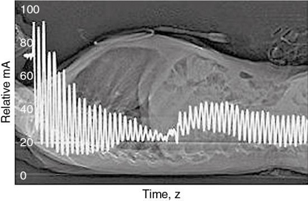
Longitudinal (z-axis) tube current modulation
Longitudinal (z-axis) tube current modulation (z-axis TCM) is based on differences in attenuation among body parts. For example, thicker body parts such as the abdomen and pelvis will attenuate the radiation more than thinner body parts, such as the head, neck, and chest regions. The technique of z-axis TCM is designed (using a specific computer algorithm) to change the mA automatically as the patient is scanned from, say, head to toe (along the z-axis) while maintaining a constant (uniform) noise level (image noise target values) for different thicknesses of body parts examined. This is clearly shown in Fig. 10.15.
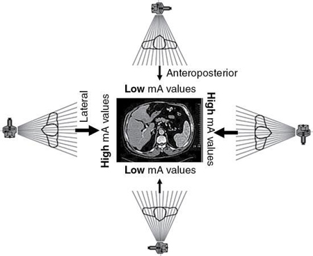
Angular (x-y axis) tube current modulation
Angular (x-y axis) tube current modulation (x-y axis TCM) is based on the fact that the radiation attenuation varies from the anteroposterior (AP) projection (low attenuation) to the lateral projection (high attenuation) as the tube rotates around (gantry rotation) the patient. Although the high-attenuation projections will require higher mA values, the low-attenuation projections will require lower mA values, as illustrated in Fig. 10.16. The x-y axis TCM algorithm ensures that a constant (uniform) noise level is maintained during the scanning process.
Angular-longitudinal tube current modulation
Fig. 10.17 illustrates a method where both x-y axis and z-axis modulation can be used together to provide the “most comprehensive approach to CT dose reduction because the x-ray dose is adjusted according to the patient-specific attenuation in all three planes” (McCollough et al., 2006).
Approaches to obtaining attenuation characteristics of the patient
The attenuation characteristics of the patient are one of the first pieces of information required to use AEC systems in CT imaging (that is, vary the mA during the scanning process and keep the image noise constant, regardless of the gantry rotation and the z-axis position). Such information is currently obtained by two different schemes. Although the first approach uses a CT scanned projection radiograph (SPR), the typical “scout view” (also referred to as ScoutView, Topogram, or the Scanogram, depending on the CT vendor), the second approach makes use of “on-line” data “from the preceding 180° of rotation to modulate the mA” (Lewis, 2005).
Defined level of image quality in CT automatic exposure control
The second requirement when AEC is used in CT imaging is that operators must set up the defined level of image quality on their respective CT scanners. The approaches from four CT vendors include a noise index (GE Healthcare), a reference image (Philips), a quality reference mAs (Siemens), and the standard deviation of CT numbers or an image quality level (Toshiba). Each of these is briefly described in Table 10.1. Essentially, the fundamental basis for these methods, rests on several important points:
- 1. A CT projection radiograph is required from which attenuation data are obtained.
- 2. An image quality index is prescribed (prescription of the mA). This index is related to the noise level (standard deviation of the CT numbers in a water phantom; Lewis, 2005).
- 3. A referenced image is selected (from previous examinations) that has the image quality required and the mA is adjusted to produce the same level of image quality as the referenced image when scanning other patients.
- 4. These methods are based on the use of proprietary algorithms.
| CT Vendor | Image Quality Paradigm | Descriptiona |
|---|---|---|
| GE Healthcare | Noise index | The noise index is referenced to the standard deviation of CT numbers within the region of interest in a water phantom of a specific size. A look-up table is then used to map the patient-specific attenuation values measured on the CT projection radiograph (scout image) to tube current values for each gantry rotation according to a proprietary algorithm. The algorithm is designed to maintain the same noise level as the attenuation values change from one rotation to the next. Different noise indices may be required for patients of different sizes. |
| Philips | Reference image | In a process that the manufacturer calls automatic current setting, the user selects an acceptable patient examination, and the system saves the image (including the raw CT projection data and the CT projection radiograph, or “surview”) as the reference data for comparison with the CT projection radiograph and data obtained from other patients in examinations for the same diagnostic task. The comparison is performed with the use of a proprietary algorithm and on a protocol-by-protocol basis (i.e., for a given examination type) to enable the automated selection of the appropriate tube current values by the scanner. |
| Siemens | Quality reference mAs | For each examination type (i.e., protocol) the user selects the effective tube current-time product (tube current-time product/pitch) typically used for a CT in a patient with a weight of approximately 80 kg. (For pediatric protocols the effective tube current-time product that should be selected is that typically used for a CT in a 20-kg patient.) The noise target (standard deviation of the CT numbers) is varied on the basis of patient size by using an empirical algorithm; thus, image noise is not kept constant for all patients but is adjusted according to an empirical impression on image quality. CT projection radiography (“topograms”) for each patient is used to predict the tube current curve (with variations along the x-y and z-axes) that will yield the desired image quality, given the patient’s size and anatomy. An on-line feedback system fine-tunes the actual tube current values during scanning to precisely match the patient-specific attenuation values at all angles (as opposed to the attenuation values estimated on the basis of one angle of the CT projection radiograph). |
| Toshiba | Standard deviation of CT numbers | Both methods are referenced to the standard deviation of CT numbers measured in a patient-equivalent water phantom. Data from the patient’s CT projection radiograph (scanogram) are used to map the selected image quality to tube current values. |
| Image quality level |
aMcCollough, M. C., Bruesewitz, M. R., & Kofler, J. M., Jr. (2006). Radiographics, 26, 503–512.
Iterative and deep learning reconstruction algorithms
Iterative reconstruction (IR) and deep learning image reconstruction (Artificial Intelligence-Based Approach) algorithms in CT were described in detail in Chapter 6 in terms of a technical overview as well as their influence on image quality and dose. In summary, the primary advantages of iterative image reconstruction and deep learning reconstruction (DLR) algorithms are to reduce image noise (in low-dose CT scanning) and minimize the higher radiation dose inherent in the filtered back-projection algorithm. All major CT manufacturers offer IR algorithms as of 2014.
In general, the IR approach uses the filtered back-projection CT image data, referred to as the measured projections, to create simulated projections, which are then compared with the initial measured projections. These comparisons are done to determine differences in image noise. Once this difference is obtained, it is applied to the simulated projection to correct for inconsistencies. A new CT image is subsequently reconstructed and the process repeats until the difference between the measured and simulated projections are minor enough to be acceptable (Kaza et al., 2014; Qiu and Seeram, 2016). IR algorithms produce images with reduced noise and artifacts. Maldjian and Goldman (2013) and Kaza et al. (2014) showed reductions in radiation dose using IR that vary from 30% to 50% (Qiu and Seeram, 2016). The studies cited have included dose reductions in pediatric studies, CT abdominal examinations, and CT angiography.
DLR algorithms on the other hand, “significantly improved image noise and the overall image quality... and offered an additional significant radiation dose reduction while allowing slices to be twice as thin as compared to hybrid-IR. Thus, DLR can yield better image quality than hybrid-IR while reducing radiation dose” (Lenfant et al., 2020). Additionally, a more recent study (Brady et al., 2020) on the use of DLR to reduce dose and improve image quality in pediatric CT using the filtered back projection (FBP), statistical-based iterative reconstruction (SBIR), and model-based iterative reconstruction (MBIR) algorithms, showed that “compared with FBP, SBIR, and MBIR, DLR demonstrated improved object detectability by 51% (16.5 of 10.9), 18% (16.5 of 13.9), and 11% (16.5 of 14.8), respectively. DLR reduced image noise without noise texture effects seen with MBIR. Radiologist ratings were 7 ± 1 (DLR), 6.2 ± 1 (MBIR), 6.2 ± 1 (SBIR), and 4.6 ± 1 (FBP); two-way analysis of variance showed a difference on the basis of reconstruction type (P <.001). Radiologists consistently preferred DLR images (intraclass correlation coefficient, 0.89; 95% CI: 0.83, 0.93). DLR demonstrated 52% (1 of 2.1) greater dose reduction than SBIR”. For a review of IR algorithms, and DLR algorithms, the interested reader should refer to Chapter 6.
Image quality and dose: Operator considerations
It is clear from the foregoing discussion that image quality and dose are closely related. Image quality includes spatial resolution, contrast resolution, and noise. Although spatial resolution depends on geometric factors (such as focal spot size, slice thickness, and pixel size, for example), contrast resolution and noise depend on both the quality (beam energy) and quantity (number of x-ray photons) of the radiation beam. Several mathematical equations have been derived to express the relationship between dose and image quality (Bushong, 2017). For CT operators, the following mathematical expression is important:
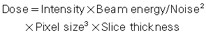
where intensity and beam energy depend on mA and kV, respectively, and noise depends on the number of photons detected and used to create the image. This expression is read as follows: dose is directly proportional to the product of mA and kV and inversely proportional to the product of noise squared, pixel size cubed, and slice thickness.
The expression also implies the following about dose and image quality:
- 1. To reduce the noise in an image by a factor of 2 requires an increase in the dose by a factor of 4.
- 2. To improve the spatial resolution (pixel size) by a factor of 2 (keeping the noise constant) requires an increase in the dose by a factor of 8.
- 3. To decrease the slice thickness by a factor of 2 requires an increase in the dose by a factor of 2 (keeping the noise constant).
- 4. To decrease both the slice thickness and the pixel size by a factor of 2 requires an increase in the dose by a factor of 16 (23 × 2 = 2 × 2 × 2 × 2).
- 5. Increasing mA and kV increase the dose proportionally. For example, a twofold increase in mA increases the dose by a factor of 2. Additionally, doubling the dose will require an increase by the square of the kV (kV2).
As stated in 5 above, the dose is proportional to kV2. This relationship often causes some difficulty for technologists in practice. As described by Reid et al. (2010) the power (2) can vary from 2.5 to 3.1 and depends on the patient’s size. Maldjian and Goldman (2013), reported that decreasing the kilovolt peak from 140 kV to 120 kV, reduced the dose by 28% to 40% for a typical phantom. The authors reported that further decreasing to 80 kV reduces the dose by approximately 65%. Precise adjustment of dose should not be obtained solely through manipulation of peak kilovoltage. Furthermore, Gill et al. (2015) showed that at 100 kV and 120 kV, the effective dose was 3.2 and 6.8 mSv, respectively, in computed tomography pulmonary angiography (CTPA). This is a significant dose reduction when operating the x-ray tube at 100 kV as opposed to 120 kV.
In yet another CT dose study by Smith-Bindman et al. (2019) the authors showed that “variation in doses used for CT scanning across patients is primarily driven by how CT scanners are used, and not to factors related to the patient, institution, or machine The large variation in doses across countries is mainly attributable to institutional decisions regarding the technical parameters that are used rather than to underlying differences in the patients scanned or the machines used These findings suggest that optimizing doses to a consistent standard is possible, which will probably require more education of individuals who create protocols for CT, recalibration of image quality expectations targeted to answering the clinical question at hand, and greater sharing of protocols across institutions.” These results lead to the next topic of importance in the CT dose picture, and that is optimization.
CT dose optimization
In this chapter so far, two points have been made clear. First, CT is rapidly expanding in its use in medicine. Second, a major concern that is receiving increasing attention in the literature relates to the potential for high radiation doses delivered by CT scanners and the potential biological risks associated with the high doses from CT examinations (Hendee & O’Connor, 2013). With these concerns in mind, there have been increasing efforts to reduce the dose to the patient without compromising the image quality needed to make a diagnosis. One such significant approach is that of dose optimization, and to date various strategies have been devised to help CT users reduce the dose to the patient while maintaining optimal image quality (Seeram & Brennan, 2017).
Biological effects of radiation exposure
Biological effects of radiation exposure were described previously. In summary, these effects fall into two broad categories: stochastic effects and deterministic effects. Stochastic effects are random, and the probability of their occurrence depends on the amount of radiation dose an individual receives. The probability increases as the dose increases, and there is no threshold dose for stochastic effects. Any amount of radiation, no matter how small, has the potential to cause harm. If harm occurs, the damage generally becomes apparent years after exposure; therefore, stochastic effects also are called late effects. Examples of stochastic effects include cancer and genetic damage (Bushong, 2017; Seeram & Brennan, 2017). Stochastic effects are considered a risk from exposure to the low levels of radiation used in medical imaging, including CT examinations.
Deterministic effects are those for which the severity of the effect (rather than the probability) increases with radiation dose and for which there is a threshold dose. Examples of deterministic effects include skin burns, hair loss, tissue damage, and organ dysfunction (Bushong, 2017). Deterministic effects are also referred to as early effects and involve high exposures that are unlikely to occur in medical imaging examinations.
Radiation protection philosophy
In diagnostic medical imaging, practitioners purposefully expose patients to a low dose of ionizing radiation as a means to improve or restore patients’ health. The goal of radiation protection is to prevent deterministic effects by ensuring that doses remain well below relevant threshold doses and to minimize the probability of stochastic effects.
To accomplish this goal, radiation protection in medical imaging is guided by international and national recommendations and frameworks such as those established by the International Commission on Radiological Protection (ICRP); and national radiation protection organizations such as the National Council on Radiation Protection and Measurements (NCRP); US Food and Drug Administration (FDA), and the Radiation Protection Bureau, Health Canada (RPB-HC), along with individual state guidelines and regulations.
The ICRP has provided three guiding principles of radiation protection (ICRP, 2007); namely, justification, optimization, and dose limitation. While the principles of justification and optimization address individuals who are exposed to radiation, the principle of dose limits deals with occupational and environmental exposures and excludes medical exposure. This subsection will only focus on the principle of optimization.
What is dose optimization?
Dose optimization is a radiation protection principle intended to ensure that doses delivered to patients are kept as low as is reasonably achievable (ALARA). The ultimate goal of optimization is to minimize stochastic effects and to prevent deterministic effects. The ICRP recommends approaches to dose optimization associated with radiography equipment and daily operations. While equipment optimization refers to the manufacturer’s design and construction of the imaging unit, operations optimization refers to the options radiologic technologists choose that enable them to follow the ALARA principle during the examination (ICRP, 2007). Optimization strategies also address image quality. Specifically, dose optimization strategies must not compromise the image quality required by physicians to diagnose diseases and conditions
Optimization strategies
As described earlier in this chapter, a number of factors affect the dose to the patient in CT. These include the scan parameters such as exposure technique factors (constant and effective mAs and kV), collimation (z-axis geometric efficiency), pitch, number of detectors, over-ranging (z-overscanning), patient centering, ATCM, and iterative and deep learning image reconstruction algorithms. In review, a brief summary of important CT dose parameters is provided in Table 10.2. To effectively reduce the dose and maintain the needed image quality parameters listed and defined in Table 10.3, users must have systematic approaches or strategies to accomplish the goals dose optimization.
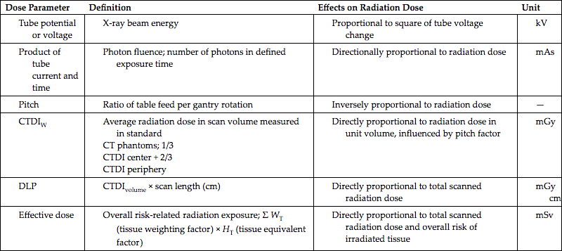
| Dose Parameter | Definition | Effects on Radiation Dose | Unit |
|---|---|---|---|
Tube potential or voltage |
X-ray beam energy |
Proportional to square of tube voltage change |
kV |
Product of tube current and time |
Photon fluence; number of photons in defined exposure time |
Directionally proportional to radiation dose |
mAs |
Pitch |
Ratio of table feed per gantry rotation |
Inversely proportional to radiation dose |
— |
CTDIW |
Average radiation dose in scan volume measured in standard CT phantoms; 1/3 CTDI center + 2/3 CTDI periphery |
Directly proportional to radiation dose in unit volume, influenced by pitch factor |
mGy |
DLP |
CTDIvolume × scan length (cm) |
Directly proportional to total scanned radiation dose |
mGy cm |
Effective dose |
Overall risk-related radiation exposure; Σ WT (tissue weighting factor) × HT (tissue equivalent factor) |
Directly proportional to total scanned radiation dose and overall risk of irradiated tissue |
mSv |
CTDI, CT dose index; DLP, dose length product.
Reprinted with permission from Goo, H. W. (2012). Korean Journal of Radiology, 13 (1), 1–11.

| Image Quality Parameter | Definition | Relationships with Radiation Dose Parameters | Calculation Method |
|---|---|---|---|
| Image noise | Random variation of CT numbers | Inversely proportional to square root of radiation dose; inversely proportional to tube voltage; inversely proportional to fourth power of spatial resolution; influenced by section thickness and reconstruction algorithm | Standard deviation of measured CT numbers |
| Contrast-to-noise resolution | Ability to distinguish between different CT numbers | Not significantly changed at different tube voltages in most of materials except for some with high atomic numbers such as iodine (increased at low tube voltage); low-contrast resolution greatly influenced by image noise level | (SA − SB)/σ, where SA and SB are CT attenuation measured in structures A and B and σ is measured image noise |
| Spatial resolution | Ability to distinguish small details of object | Inversely proportional to focal spot size, detector collimation; influenced by reconstruction algorithm | Voxel size; line pairs per centimeter; point or line spread function; modulation transfer function |
| Artifacts | Unwanted structures degrading CT image quality | Photon starvation artifacts—inversely proportional to radiation dose; physiologic motion artifacts—inversely proportional to temporal resolution; other artifacts—no direct relationships with radiation dose parameters | — |
Reprinted with permission from Goo, H. W. (2012). Korean Journal of Radiology, 13 (1), 1–11.
In the past, several authors have described various dose optimization strategies in CT, especially in MSCT, that are not significantly different than more recent optimization strategies (Parakh et al., 2016; Smith-Bindman & Boone, 2014; Thakur et al., 2013). It is not within the scope of this chapter to describe details of these strategies; however, it is noteworthy to highlight a few essential guiding principles. Several strategies that emerge as common themes relate to the mAs, kV, collimation, slice thickness, scanned volume, pitch, and the use of ATCM techniques. A notable checklist for dose optimization is provided in Table 10.4.
Reprinted with permission from Goo, H. W. (2012). Korean Journal of Radiology, 13 (1), 1–11.
Research on dose optimization and image quality1
Dose optimization in CT based on image quality requires a thorough understanding of CT dose parameters and CT image quality parameters. CT image quality has been described in terms of high-contrast spatial resolution, low-contrast resolution, temporal resolution, CT number accuracy and uniformity, image noise, and image artifacts. Research has continued to determine the best methods for lowering radiation dose in CT examinations without compromising the diagnostic quality of images. These studies often are complex so they can follow precise scientific methods, including identifying the problem, performing a literature review, stating the goals regarding investigation of the problem, and designing a methodology to find a solution to the problem. Scientific methods also include data collection, analysis and interpretation of the data, and dissemination of the study findings.
In general, research on optimizing dose and image quality involves various methodologies to demonstrate dose reduction without a loss of image quality. To determine optimal image quality, McCollough et al. (2006) stressed that studies must involve quantitative metrics such as image noise and observer performance
In a special issue of the journal Radiation Protection Dosimetry dedicated to optimization strategies in medical imaging for fluoroscopy, radiography, mammography, and CT, several studies identified at least four important requirements for dose and image quality optimization research (Mattsson, 2005):
- 1. Ensure patient safety.
- 2. Determine the level of image quality required for a particular diagnostic task.
- 3. Acquire images at various exposure levels from high to low and in such a manner that accurate diagnosis can still be made.
- 4. Use reliable and valid methodologies for the dosimetry, image acquisition, and evaluation of image quality using human observers, remembering the nature of the detection task.
To accomplish these requirements, CT dose and image quality optimization studies should generally ensure that the following minimum essential elements are considered:
- 1. The CT imaging system is calibrated to ensure consistent and reliable performance.
- 2. The dosimeters used to capture dose levels are calibrated.
- 3. Researchers use appropriate phantoms (anthropomorphic phantoms and phantoms for determining objective image quality parameters [Zarb et al., 2010]) and acceptable dose measurement methodology of acquiring scans at different exposure levels.
- 4. Images are assessed in two phases:
- A. Expert observers evaluate image quality based on a defined and specific criterion (such as the appearance of image noise) to establish an optimized dose level.
- B. The same set of observers is used to assess images obtained at various dose levels, including an optimized dose level, using established, valid, and reliable observer performance methods. Observer performance methods include receiver-operating characteristic (Zarb et al., 2010) and visual grading analysis (Tingberg et al., 2005) methods. The task of pathology detection requires a different observer performance test than that of detecting normal anatomical structures.
Receiving-operator characteristic is the most common observer performance method. Under this method, a study’s observers determine whether an image contains a lesion or pathology. The observer assigns a grade on a scale (e.g., 1 to 5) that rates the observer’s level of confidence in the decision (Tingberg et al., 2005).
A visual grading analysis assigns a grade to the image’s quality based on comparison with a reference image. Visual grading analysis is based on the assumption that an observer’s ability to see and evaluate normal anatomy correlates to the ability to evaluate pathology, or abnormal findings (Tingberg et al., 2005).
Radiation protection considerations
The dose optimization strategies described so far focus on methods to reduce the dose to the patient. What about the protection of personnel in CT scanning? Radiation protection of both patients and personnel in medicine is guided by two triads that are intended to ensure that medical radiation workers work within the ALARA philosophy of the ICRP. One triad deals with radiation protection actions, and the other triad addresses the radiation protection principles (Seeram and Brennan, 2017).
Radiation protection actions
Radiation protection actions include the use of time, shielding, and distance, which are intended to protect both patients and personnel in radiology. For example, because dose is proportional to the time of exposure, to protect personnel in CT, it is essential to minimize the time spent in the CT scan room during the exposure. Distance, on the other hand, is a major dose reduction action because the dose is inversely proportional to the square of the distance. This means that the further one is away from the radiation source, the less the dose received. In CT, because the patient is the main source of scatter, technologists should stand back as far away from the patient as possible if is necessary to be in the scan room during scanning. This implies that a power injector that can be controlled from outside the scan room is recommended. If a hand injector is used, then long tubing should be included.
Shielding is intended to protect not only patients (gonadal, breast, eyes, and thyroid) but also personnel and members of the public. Patients are often concerned about the exposure of their gonads during a CT examination. Because most of the gonadal exposure will come from internal scatter and not from the primary beam (unless the gonadal region was being examined), there is no need for this concern. Technologists, however, depending on the CT department policies, may place gonadal shielding on the patient because it may alleviate any fears about the risks of exposure to radiation. Shields can also be used to protect the eyes, breast, and thyroid of patients undergoing CT examinations. Bismuth shielding in CT has received some attention as to their effectiveness in offering protection, hence, the next section will provide a glimpse into the current state-of-the-art with respect to their use in CT.
Bismuth shielding in CT
Use of bismuth shield for protection of superficial radiosensitive organs
The use of bismuth (Bi) shields in CT has been discussed in recent literature reviews for protection of radiosensitive organs, most notably the breast, by attenuating the primary radiation beam from the x-ray tube (Lawrence & Seeram, 2017; Mehnati et al., 2019). Lawrence and Seeram (2017) found that “while bismuth shielding proves to provide significant dose reductions to radiosensitive organs, numerous concerns exist including wasted radiation, reduced image quality and unpredictable results when combined with AEC. Alternative methods such as tube current modulation and iterative reconstruction algorithms can provide equivalent dose savings at superior image quality, without the limitations of bismuth shields. Until these alternative methods become available in all departments, bismuth shielding remains a viable dose reduction strategy.”
The recent review by Mehnati et al. (2019) concluded that “the presence of a Bi shield was effective to decrease the patients’ surface radiation dose by decreasing the low-energy photons delivered at the surface. Comparison among the doses to the eye, thyroid, and breast showed that Bi shielding has potential for use in dose reduction, especially at the thyroid, without significantly lowering the image quality. Image quality, usage of foam, beam energies, and backscatter radiation were important factors that directly affected the efficacy of Bi shielding. The image noise assessed for imaging with and without Bi shield indicated that the increase in the noise level under Bi shielding was acceptable for making the diagnosis. Additionally, foam of optimum 1–2 cm thickness was recommended to decrease the noise in images acquired with bismuth shielding.”
The use of bismuth shields in CT discussed in the literature has sparked some debate among academics and practitioners, and various studies have shown advantages in dose reduction as well as problems imposed by these shields during the examination. This has led the AAPM to issue the following Position Statement on the Use of Bismuth Shielding for the Purpose of Dose Reduction in CT scanning (AAPM, 2014). The following statement is “policy text”:
“Bismuth shields are easy to use and have been shown to reduce dose to anterior organs in CT scanning. However, there are several disadvantages associated with the use of bismuth shields, especially when used with automatic exposure control or tube current modulation. Other techniques exist that can provide the same level of anterior dose reduction at equivalent or superior image quality that do not have these disadvantages. The AAPM recommends that these alternatives to bismuth shielding be carefully considered, and implemented when possible.”
The AAPM also provides a description of the reason for this policy, and lists the following disadvantages of using bismuth shields. These include:
- 1. “Applying bismuth shielding together with automatic exposure controls (AEC) systems, such as tube current modulation (TCM), leads to unpredictable and potentially undesirable levels of dose and image quality.
- 2. The shields can degrade image quality and accuracy.
- 3. The shields waste some of the patient’s radiation exposure.”
Furthermore, the AAPM also provides “Alternative methods for reducing dose to peripheral organs in CT scanning” and lists 14 references of relevance to the use of bismuth shielding in CT. The interested reader should refer to this AAPM document.
In order to improve the performance of bismuth shields in terms of dose reduction in CT,
Noor Azman et al. (2016) and Abunahel et al. (2018) applied bismuth oxide (Bi2O3) nanoparticles (instead of micro particles) and silicone rubber to make a nano bismuth shield to improve the efficiency of the shield in reducing the radiation dose to radiosensitive organs. Subsequently, Mehnati et al. (2020) showed that the nano Bi2O3 shield (instead of micro bismuth shield) with 1mm thickness, reduced the dose by about 15% higher. Furthermore, the noise increase in nano Bi2O3 shields was equal to 14%, which is less than the micro bismuth shield. They concluded that “the nano bismuth composite shield with different ratios and thicknesses show significant dose reduction in the breast. This could play a role in breast cancer prevention during chest CT scan.”
In yet another study examining the quantification of CT numbers (CTN) and the contrast-to-noise ratios (CNRs) “for five tissue-mimicking materials for bismuth shields of different thicknesses and for positions relative to these shields during CT scans” and dose reduction for different thicknesses of bismuth shields, Liao et al. (2019) found that “using a bismuth shield could result in significant CTN changes and perceivable artefacts, particularly for a superficial organ close to the shield, and is not recommended for quantification CT examinations or follow-up CT examinations.”
CT room shielding: Brief overview
When personnel are expected to be present in the CT scan room during the exposure, lead aprons should be worn (for the same reason that gonadal shields are placed on patients) because of the presence of scatter (Bushong, 2017).
Because scatter radiation is present during a CT examination and strikes the walls of the CT room, these walls should be shielded to protect members of the public or other radiation workers who are present outside the room. The use of minimum shielding in the form of thick plate-glass control room viewing windows and gypsum wall board with no lead content can sometimes provide the minimum required shielding. The interested reader may refer to Seeram (2020) and Seeram and Brennan (2017) for an overview of the design of protective barriers in x-ray rooms, and to Sutton et al. (2020) for more detailed information on shielding of CT scanner rooms.
The role of the CT technologist
The technologist must always observe the ALARA principle when conducting CT examinations, and must play a significant role in optimizing the dose in CT for several reasons, such as acquiring the images from the patient and paying attention to all aspects of the examination, including patient communication, patient positioning and care, technical aspects of data acquisition and image reconstruction, as well as radiation protection considerations, and so on.
Seeram (2014) provided a list of factors to which the technologist must pay careful attention when optimizing the image quality and dose in CT. These include:
- 1. The risks of radiation and CT dose in particular.
- 2. Current technical advances in CT.
- 3. CT dose metrics, particularly CTDIvolume, the DLP and effective dose, and associated units.
- 4. CT image quality metrics such as spatial resolution, contrast resolution, noise, and artifacts.
- 5. The technical factors affecting patient dose in CT, including exposure technique factors ([kVp and mAs], AEC, pitch, effective mAs, slice thickness, SFOV, beam collimation, noise-reducing algorithms [IR algorithms], anatomical coverage, overbeaming and over-ranging, patient centering, and noise index).
- 6. Scan protocols and reviewing the protocols with the radiologist on an ongoing basis with the goal of optimizing dose and image quality.
- 7. The prescan and postscan display of CT dose reports showing the CTDIvolume, the DLP, and effective dose.
- 8. How to get involved with the development or implementation of a CT dose-monitoring or dose-tracking system for the technologist’s CT department. Monitoring and tracking should include items such as dose capture, conversion of absorbed dose to effective dose, patient-specific storage, dose analytics, dose communication, and data export.
- 9. How to participate in research on CT patient dose and image quality optimization. This requires a fundamental knowledge of CT equipment and dosimeter calibration, image acquisition details, observer performance measures, and appropriate statistical tools.
- 10. How to ensure continuous professional development through relevant continuing education activities.
Diagnostic reference levels: A useful tool for optimization
Definition
The term diagnostic reference level (DRL) was first introduced by the ICRP in 1990, and subsequently explained in more detail in 1996, and updated in 2017 (ICRP, 2017). In this updated publication, the ICRP recommends the use of the following:
“A DRL is a form of investigation level used to aid in optimisation of protection in the medical exposure of patients for diagnostic and interventional procedures. A DRL value is a selected level of a DRL quantity for broadly defined types of equipment for typical examinations for groups of patients within an agreed weight range or, in certain specific circumstances, a standard phantom. DRLs do not apply to individual patients. They are derived as an arbitrary threshold from radiation metric data obtained locally and collected nationally or regionally. A DRL is a supplement to professional judgement and does not provide a dividing line between good and bad medical practice. All individuals who have a role in subjecting a patient to a medical exposure should be familiar with DRLs as a tool for optimisation of protection.”
DRLs are now used globally and have been endorsed by various organizations such as the ICRP, the American College of Radiology (ACR), the AAPM, United Kingdom Health Protection Agency, International Atomic Energy Agency, and European Commission (Seeram & Brennan, 2017). There are several reasons why it is important to implement DRLs. It is not within the scope of this chapter to outline these reasons in any detail; however, it is noteworthy that these reasons address legal or regulatory requirements, societal benefits, and improved awareness of radiation doses (Seeram & Brennan, 2017).
Establishing DRLs
There are several steps to establishing DRLs (ICRP, 2017; Seeram & Brennan, 2017). First, DRLs must be relevant to the state or country where they are applied. To be relevant, DRLs are determined from radiation dose survey data. The aggregate data from these surveys represent all hospitals in a particular region or state. Dose surveys should be performed by hospitals continuously or at least regularly carried out in three to five consecutive annual intervals. DRLs should be considered a dynamic and changing parameter so that they are always applicable to examinations performed or to new hospital equipment.
When planning a dose survey, a number of parameters should be considered: examination type, number and type of hospitals involved, phantom investigations, patient investigations, dosimetry methods, establishment of the reference level, and accessory information. These parameters will not be described here; however, the interested reader may refer to the ICRP Report 135 (2017) or to Seeram and Brennan (2017).
Setting DRL values
Fig. 10.18 illustrates hypothetical data collected from a survey of 17 hospital CT scanner rooms showing the doses (mGy) delivered for an AP lumbar spine projection. The dose values were arranged in increasing order. The next step is to establish DRLs. In this regard the ICRP (2017) recommends that “the median value (not the mean value) for the DRL quantity from each of the facilities in the survey should be used,” and that national DRL values should be set as the 75th percentile (see Fig 10.18). This value becomes the reference level. It is clear from Fig. 10.18, that four hospitals are above this level. This means that the four hospitals above this level need to engage in radiation protection activities that would bring the dose levels below the 75th percentile. For a thorough description of setting DRL values, the interested reader should refer to the ICRP Report 135 (ICRP, 2017).

The ACR DRL benchmarks for patient-based adult CT were established using the CTDIvolume, SSDE, and the DLP from the ACR’s Dose Index Registry. For example, the DRLs for chest without contrast, are 12 mGy (CTDIvolume); 15 mGy (SSDE); and 443 mGy-cm (DLP), while the achievable doses (AD) are 9 mGy (CTDIvolume); 11 mGy (SSDE); and 334 mGy-cm (DLP). For the abdomen and pelvis without contrast, for example, the DRLs are 16 mGy (CTDIvolume); 19 mGy (SSDE); and 781 mGy-cm (DLP), while the ADs are 13 mGy (CTDIvolume); 15 mGy (SSDE); and 639 mGy-cm (DLP) (ACR, 2018).
CT dose index registry
What is the dose index registry?
The ACR (https://www.acr.org/Practice-Management-Quality-Informatics/Registries/Dose-Index-Registry) describes the dose index registry (DIR) as a data registry that:
“....lets facilities compare their CT dose indices to regional and national values. They receive quarterly feedback reports comparing their results to aggregate results by body part and exam type.”
The menu features clinical resources; advocacy and economics; lifelong learning and CME; practice management and informatics; member resources; and research. Furthermore, the website also features information on how to participate; how to submit data; core documents; and related resources.
Review questions
Answer the following questions to check your understanding of the materials studied.
- 1. Which of the following best describes the beam geometry for single-slice spiral/helical CT scanners?
- 2. The dose distribution in CT for a single slice is given by the function:
- 3. The easiest and probably the most accurate method of measuring the dose in CT is:
- 4. The average dose to the patient from a series of scans is the:
- 5. The area under typical dose distribution profile for a single scan divided by the slice width is the:
- 6. The quantity measured by the pencil ionization chamber technique is the:
- 7. The dose to the patient in CT is affected by:
- 8. The dose to the patient is increased if:
- 9. Which of the following will decrease the MSAD to the patient in a CT examination?
- 10. Which of the following concept/principle/action deals with the intelligent use of radiation as a radiation protection measure?
References
Abunahel B.M, Ramli R.M, Quffa K.M. & Azman N.Z.N. Effect of nanofibrous porosity on the X-ray attenuation properties of electrospunn-Bi2O3/epoxy–polyvinyl alcohol (PVA) nanofiber mats Applied Physics A 8, 2018;124: doi:10.1007/s00339-018-1975-9.
AAPM REPORT NO. 111 Comprehensive methodology for the evaluation of radiation dose in X-ray computed tomography. Report of AAPM Task Group 111: The Future of CT Dosimetry. College Park, MD: AAPM.
American College of Radiology. (2018) ACR–AAPM–SPR Practice parameter for diagnostic reference levels and achievable doses in medical imaging. Retrieved from https://www.acr.ogr/-/media/ACR/Files/Practice-Parameters/diag-ref-levels.pdf. Accessed November 2020.
Amis E.S. & Jr. CT radiation dose: Trending in the right direction Radiology 1, 2011;261: 5-8 doi:10.1148/radiol.11111319.
Barreto I, Lamoureux R, Olguin C., et al. Impact of patient centering in CT on organ dose and the effect of using a positioning compensation system: Evidence from OSLD measurements in postmortem subjects Journal of Applied Clinical Medical Physics 6, 2019;20: 141-151 doi:10.1002/acm2.12594.
Berrington de Gonzalez A, Mahesh M, Kim K.P., et al. Projected cancer risks from computed tomographic scans performed in the United States in 2007 Archives of Internal Medicine 22, 2009;169: 2071-2077 doi:10.1001/archintern med.2009.440.
Blum A, Gillet R, Rauch A., et al. 3D reconstructions, 4D imaging and postprocessing with CT in musculoskeletal disorders: Past, present and future Diagnostic and Interventional Imaging 11, 2020;101: 693-705 https://doi.org/10.1016/j.diii.2020.09.008.
Boone J.M. The trouble with the CTDI100 Medical Physics 2007;34: 1364-1371.
Brady S.L, Trout A.T, Somasundaram E, Anton C.G, Li Y. & Dillman J.R. Improving image quality and reducing radiation dose for pediatric CT by using deep learning reconstruction Radiology 1, 2021;298: 180-188 https://doi.org/10.1148/radiol.2020202317.
Brenner D.J. & Hall E.J. Computed tomography: An increasing source of radiation exposure New England Journal of Medicine 22, 2007;357: 2277-2284.
Brenner D.J. It is time to retire the computed tomography dose index (CTDI) for CT quality assurance and dose optimization Medical Physics 2006;33: 1189-1191.
Brisse H.J, Madec L, Gaboriaud G., et al. Automatic exposure control in multichannel CT with tube current modulation to achieve a constant level of image noise: Experimental assessment on pediatric phantoms Medical Physics 2007;34: 3018-3032.
Bushberg A.T, Seibert J.A, Leidholdt E.M. & JrBoone J.M. The essential physics of medical imaging 3rd ed. 2012; Lippincott-Williams Philadelphia, PA.
Bushong S. Radiologic science for technologists 11th ed. 2017; Mosby-Year Book St. Louis, MO.
Cody D. & McNitt-Gray M. CT image quality and patient radiation dose: Definitions, methods, and trade-offs 2006; Radiological Society of North America Chicago, IL.
Eid M, De Cecco1 C.N, Nance J.W. & Jret al. Cinematic rendering in CT: A novel, lifelike 3D visualization technique American Journal of Roentgenology 2017;209: 370-379.
Euler A, Saltybaeva N. & Alkadhi H. How patient off-centering impacts organ dose and image noise in pediatric head and thoracoabdominal CT European Radiology 12, 2019;29: 6790-6793 doi:10.1007/s00330-019-06330-5.
Feng L.B, Pines J.M, Yusuf H.R. & Grosse S.D. U.S. trends in computed tomography use and diagnoses in emergency department visits by patients with symptoms suggestive of pulmonary embolism, 2001–2009 Academic Emergency Medicine 10, 2013;20: 1033-1040 doi:10.1111/acem.12221.
Gill M.K, Vijayananthan A, Kumar G, Jayarani K, Ng K.H. & Sun Z. Use of 100 kV versus 120 kV in computed tomography pulmonary angiography in the detection of pulmonary embolism: Effect on radiation dose and image quality Quantitative Imaging in Medicine and Surgery 4, 2015;5: 524-533 https://doi.org/10.3978/j.issn.2223-4292.2015.04.04.
Gottumukkala R.V, Kalra M.K, Tabari A, Otrakji A. & Gee M.S. Advanced CT techniques for decreasing radiation dose, reducing sedation requirements, and optimizing image quality in children RadioGraphics 2019;39: 709-726 https://doi.org/10.1148/rg.2019180082.
Haaga J.R, Miraldi F, MacIntyre W, LiPuma J.P, Bryan P.J. & Wiesen E. The effect of mAs variation upon computed tomography image quality as evaluated by in vivo and in vitro studies Radiology 1981;138: 449-454.
Hedgire S.S, Baliyan V, Ghoshhajra B.B. & Kalra M.K. Recent advances in cardiac computed tomography dose reduction strategies: A review of scientific evidence and technical developments Journal of Medical Imaging 3, 2017;4: 031211.
Hendee W.R. & O’Connor M.K. Radiation risks in medical imaging: Separating fact from fantasy Radiology 2, 2013;264: 312-320.
Hermann, T. L, Fauber, TL, Gill, J.et al. (2014) Best practices in digital radiography. Retrieved from http://asrt.org/docs/default-source/whitepapers/asrt12_bstpracdigradwhp_final.pdf?sfvrsn=4. Accessed April 9, 2014.
Hricak H, Brenner D.J, Adelstein S.J., et al. Managing radiation use in medical imaging: A multifaceted challenge Radiology 3, 2011;258: 889-905 doi:10.1148/radiol.10101157.
International Electrotechnical Commission (IEC). Particular requirements for the safety of X-ray equipment for CT 2nd ed. 2001; 60601-2-44.
International Commission on Radiological Protection (ICRP). Diagnostic reference levels in medical imaging. ICRP Publication 135 Ann ICRP 2017;46: (1).
International Commission on Radiological Protection (ICRP) Publication 103. The 2007 recommendations of the International Commission on Radiological Protection Annals of the ICRP 2–4, 2007;37: 1-332.
Isa I.N.C, Rahmat S.M.S, Dom S.M, Kayun Z. & Karim M.K.A. The effects of mis-centering on radiation dose during CT head examination: A phantom study Journal of X-ray Science and Technology 4, 2018;27: 631-639 doi:10.3233/XST-190491.
Kaasalainen T, Palmu K, Reijonen V. & Kortesniemi M. Effect of patient centering on patient dose and image noise in chest CT American Journal of Roentgenology 1, 2014;203: 123-130 doi:10.2214/AJR.13.12028.
Kalender W, Wolf H. & Suess C. Dose reduction in CT by anatomically adapted tube current modulation. II. Phantom measurements Medical Physics 1999;26: 2248-2253.
Kalra M.K, Maher M.M, Toth T.L., et al. Strategies for CT radiation dose optimization Radiology 2004;230: 619-628.
Kaza R.K, Platt J.F, Goodsitt M.M., et al. Emerging techniques for dose optimization in abdominal CT Radiographics 1, 2014;34: 4-17.
Kwan A.C, Pourmorteza A, Stutman D, Bluemke D.A. & Lima J.A.C. Next-generation hardware advances in CT: Cardiac applications Radiology 2021;298: 3-17 https://doi.org/10.1148/radiol.2020192791.
Lawrence S. & Seeram E. The current use and effectiveness of bismuth shielding in computed tomography: A systematic review Radiology – Open Journal 1, 2017;2: 7-16 doi:10.17140/ROJ-2-113.
Lell M.M, Wildberger J.E, Alkadhi H, Damilakis J. & Kachelriess M. Evolution in computed tomography: The battle for speed and dose Investigative Radiology 9, 2015;50: 629-644 doi:10.1097/RLI.0000000000000172.
Lenfant M, Chevallier O, Comby P.O., et al. Deep learning versus iterative reconstruction for CT pulmonary angiography in the emergency setting: Improved image quality and reduced radiation dose Diagnostics 8, 2020;10: 558.
Lewis M. Radiation dose issues in multi-slice CT scanning 2005; London St. George’s Hospital.
Liao Y.L, Lai N.L, Tyan Y.S. & Tsai H.S. Bismuth shield affecting CT image quality and radiation dose in adjacent and distant zones relative to shielding surface: A phantom study Biomedical Journal 5, 2019;42: 343-351.
Li J, Udayasankar U.K, Toth T.L., et al. Automatic patient centering for MDCT: Effect on radiation dose American Journal of Roentgenology 2007;188: 547-552.
Litmanovich D.E, Tack D.M, Shahrzad M. & Bankier A.A. Dose reduction in cardiothoracic CT: review of currently available methods Radiographics 2014;34: 1469-1489.
Maldjian P.D. & Goldman A.R. Reducing radiation dose in body CT: Primer on dose metrics and key CT technical parameters American Journal of Roentgenology 4, 2013;200: 741-747.
Mathews J.D, Forsythe A.V, Brady Z., et al. Cancer risk in 680,000 people exposed to computed tomography scans in childhood or adolescence: Data linkage study of 11 million Australians BMJ 2013;346: 1-18 doi:10.1136/bmj.f2360.
Mattsson S. Optimization strategies in medical X-ray imaging Radiation Protection Dosimetry 1–3, 2005;114: 1-3.
McCollough C.H, Bruesewitz M.R, Kofler J.M. & Jr. CT dose reduction and dose management tools: overview of available options Radiographics 2006;26: 503-512.
McNitt-Gray M. Tube current modulation approaches: Overview, practical issues and potential pitfalls 2011; AAPM. AAPM 2011 Summit on CT Dose. AAPM Alexandria, VA.
McNitt-Gray M.F. Radiation dose in CT Radiographics 2002;22: 1541-1553.
Mehnati P, Malekzadeh R. & Sooteh M.Y. Use of bismuth shield for protection of superficial radiosensitive organs in patients undergoing computed tomography: A literature review and meta-analysis Radiological Physics and Technology 2019;12: 6-25 https://doi.org/10.1007/s12194-019-00500-2.
Mehnati P, Malekzadeh R, Baharak Divband B. & Sooteh M.Y. Assessment of the effect of nano composite shield on radiation risk prevention to breast during computed tomography Iranian Journal of Radiology 1, 2020;17: e96002. doi:10.5812/iranjradiol.96002.
Moore W.H, Bonvento M. & Olivieri-Fitt R. Comparison of MDCT radiation dose: A phantom study American Journal of Roentgenology 2006;187: W498-W502.
Noor Azman N.Z, Musa N.F, Nik Ab Razak N.N., et al. Effect of Bi 2 O 3 particle sizes and addition of starch into Bi 2 O 3 –PVA composites for X-ray shielding Applied Physics A 9, 2016;122: 818. doi:10.1007/s00339-016-0329-8.
Papadakis A.E. CT dose optimization Physica Medica 3, 2016;32: 189. https://doi.org/10.1016/j.ejmp.2016.07.331.
Papadakis A.E. & Damilakis J. Automatic tube current modulation and tube voltage selection in pediatric computed tomography Investigative Radiology 5, 2019;54: 265-272 doi:10.1097/RLI.0000000000000537.
Parakh A, Kortesniemi M. & Schindera S.T. CT radiation dose management: A comprehensive optimization process for improving patient safety Radiology 3, 2016;280: 663-673.
Paulo G, Damilakis J, Tsapaki V., et al. Diagnostic reference levels based on clinical indications in computed tomography: A literature review Insights Imaging 2020;11: 96. https://doi.org/10.1186/s13244-020-00899-y.
Qiu D. & Seeram E. Does iterative reconstruction improve image quality and reduce dose in computed tomography? Radiology – Open Journal 2, 2016;1: 42-54 doi:10.17140/ROJ-1-108.
Reid J, Gamberoni J, Dong F. & Davros W. Optimization of kVp and mAs for pediatric low dose simulated abdominal CT: Is it best to base parameter selection on object circumference? American Journal of Roentgenology 4, 2010;195: 1015.
Rubin G.D. Computed tomography: Revolutionizing the practice of medicine for 40 years Radiology Suppl. 2, 2014;273: S45-S74.
Saltybaeva N. & Alkadhi H. Vertical off-centering affects organ dose in chest CT: Evidence from Monte Carlo simulations in anthropomorphic phantoms Medical Physics 11, 2017;44: 5697-5704 doi:10.1002/mp.12519.
Seeram E. Rad Tech’s guide to radiation protection 2020; Wiley and Sons Ltd Hoboken, NJ.
Seeram E. & Brennan P.C. Radiation protection in diagnostic X-ray imaging 2017; Jones and Bartlett Learning Burlington, MA.
Seeram E. Computed tomography dose optimization Radiologic Technology 6, 2014;85: 665-675.
Smith-Bindman R, Kwan M.L, Marlow E.C., et al. Trends in use of medical imaging in US health care systems and in Ontario, Canada, 2000–2016 JAMA 9, 2019;322: 843-856 doi:10.1001/jama.2019.11456.
Smith-Bindman R, Wang Y, Chu P., et al. International variation in radiation dose for computed tomography examinations: Prospective cohort study BMJ 2019;364: k4931. doi:10.1136/bmj.k4931.
Smith-Bindman R. & Boone J.M. Introduction to the special issue: Radiation dose optimization—Improving the safety of CT Journal of the American College of Radiology: JACR 3, 2014;11: 229-230.
Supanich M.P. Tube current modulation 2013; AAPM Alexandria, VA 3rd CT Dose Summit. Strategies for CT Scan Parameter Optimization. AAPM.
Sutton, D, Collins, L. T, & Le Heron, J (2020). Chapter 24: Radiation protection/shielding in computed tomography. Diagnostic Radiology Physics: A Handbook for Teachers and Students. IAEA. Retrieved from https://humanhealth.iaea.org/HHW/MedicalPhysics/TheMedicalPhysicist/Studentscorner/HandbookforTeachersandStudents/Chapter_24.pdf. Accessed November 2020.
Thakur Y, McLaughlin P.D, John R. & Mayo J.R. Strategies for radiation dose optimization Current Radiology Reports 2014;1: 1-10 doi:10.1007/s40134-013-0007-y.
Tingberg A, Båth M, Håkansson M., et al. Evaluation of image quality of lumbar spine images: A comparison between FFE and VGA Radiation Protection Dosimetry 1–3, 2005;114: 53-61.
Toth T, Ge Z. & Daly M.P. The influence of patient centering on CT dose and image noise Medical Physics 2007;34: 3093-3101.
Tsujiguchi T, Obara H, Ono S, Saito Y. & Kashiwakura I. Consideration of the usefulness of a size-specific dose estimate in pediatric CT examination Journal of Radiation Research 4, 2018;59: 430-435 https://doi.org/10.1093/jrr/rry022.
Tzedakis A, Damilakis J, Perisinakis K., et al. Influence of z overscanning on normalized effective doses calculated for pediatric patients undergoing multidetector CT examinations Medical Physics 2007;34: 1163-1172.
Van der Molen A.J, Stoop P, Prokop M. & Geleijns J. A national survey on radiation dose in CT in The Netherlands Insights Imaging 3, 2013;4: 383-390 doi:10.1007/s13244-013-0253-9.
Van der Molen A.J. & Geleijns J. Overranging in multisection CT: Quantification and relative contribution to dose—Comparison of four 16-section CT scanners Radiology 2007;242: 208-216.
Waszczuk L.A, Guziński M, Czarnecka A. & Sąsiadek M.J. Size-specific dose estimates for evaluation of individual patient dose in CT protocol for renal colic American Journal of Roentgenology 2015;205: 100-105.
Wolbarst A.B, Capasso P. & Wyant A.R. Medical imaging: Essentials for physicians 2013; Wiley-Blackwell Hoboken, NJ.
Yurt A, Özsoykal İ. & Obuz F. Effects of the use of automatic tube current modulation on patient dose and image quality in computed tomography Molecular imaging and Radionuclide Therapy 3, 2019;28: 96-103 https://doi.org/10.4274/mirt.galenos.2019.83723.
Zarb F, Rainford L. & McEntee M.F. Image quality assessment tools for optimization of CT images Radiography 2010;16: 147-153.