12: Multislice computed tomography: Physical principles and instrumentation
Learning objectives
On completion of this chapter, you should be able to:
- 1. discuss the controversy surrounding the use of the terms “spiral” and “helical” in volume CT.
- 2. outline the scanning sequence of conventional CT and list its principal limitations.
- 3. list the requirements for volume data acquisition.
- 4. outline the physical principles, data acquisition, and image reconstruction technique for single-slice spiral/helical CT.
- 5. describe the major equipment components of a single-slice spiral/helical CT scanner.
- 6. define and explain briefly each of the following:
- • pitch
- • volume coverage
- • collimation and table speed
- • scan time
- • reconstruction increment.
- 7. describe the essential elements of image quality and radiation dose for single-slice spiral/helical CT.
- 8. state the advantages and limitations of single-slice spiral/helical CT.
- 9. briefly explain three major technical advances in volume CT scanning.
- 10. describe the essential characteristics of multi-slice detectors.
- 11. state the limitations of single-slice volume CT scanning.
- 12. trace the evolution of multislice volume CT scanners.
- 13. compare and contrast data and image reconstruction for single-slice and multislice volume CT, including cone-beam algorithms.
- 14. describe the essential features of each of the following equipment components:
- • data acquisition components
- • multislice detectors
- • slice thickness selection
- • data acquisition system
- • patient table
- • computer system.
- 15. define and explain the goals of isotropic imaging.
- 16. describe the main technical aspects of wide area detector CT.
- 17. outline the major technical components of the dual-source CT scanner.
- 18. state the advantages of multislice spiral/helical CT.
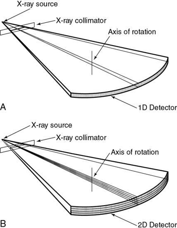
In 1990, the first computed tomography (CT) scanner to perform volume data acquisition was introduced (Kalender, 1995). This scanner was invented to overcome the problems imposed by conventional (slice-by-slice axial sequential scanning) CT scanners. Furthermore, the scanners provide shorter scan times to sub-second levels and improvement in three-dimensional (3D) imaging. These scanners are referred to as single-slice spiral/helical CT scanners or volume CT scanners on the basis of the beam geometry (spiral/helical) used during the data acquisition process. The term single-slice CT (SSCT) will be used in this chapter to refer to CT scanners that acquire a volume dataset by scanning a volume of the patient’s anatomy using a 1D detector array, as opposed to the conventional CT scanner that obtains a single dataset using a 1D detector array. Subsequent developments and advances in CT technology have led to the introduction of multislice CT (MSCT) scanners that now acquire volume datasets (much faster than SSCT scanners) using 2D detector arrays. MSCT scanners are now commonplace and have replaced SSCT scanners. It is important to note that some authors prefer to use the term multidetector CT (MDCT) on the basis of the design of the 2D detector arrays. The acronym MSCT will be used throughout this text.
The purpose of the chapter is threefold. First, the language of SSCT scanning will be introduced followed by a description of the fundamental principles and concepts of spiral/helical data acquisition, image reconstruction, major system components, basic scan parameters, and the advantages and limitations of SSCT scanners. Second, the evolution of MSCT scanners will be highlighted, followed by a description of the physical principles and technology of MSCT scanners. The technical principles and concepts of SSCT scanners described in this chapter lay the foundations necessary for a good understanding of MSCT scanners. The third goal of this chapter is to list the clinical applications of MSCT.
SSCT: Historical background
The development of spiral/helical CT principles dates back several decades, with significant contributions from several notable individuals. An early pioneer in the development of the technique of volume scanning in CT was Dr. Willi A. Kalender (see Chapter 1) of the Institute of Medical Physics at the University of Erlangen, Germany. Kalender started work on spiral CT in 1988 with Peter Vock from Switzerland, and in 1989 he described the technical details and clinical applications of spiral CT to the Radiological Society of North America (RSNA) meeting in Chicago. Other early investigators included Mori (1987), various Japanese researchers, such as Tohki, (1991); Taguchi & Aradate, 1998; Saito, (1998); Hu, 1999; and He, (1999). Furthermore, additional early pioneers included Feldkamp, Davis, Kress (1984); Bresler and Skrabacz (1993); and Liang and Kruger (1996). These pioneers have been cited in this chapter since it is essential that their work be recognized and their papers considered as seminal information.
Terminology controversy
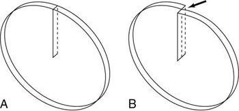
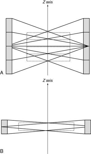
Kalender and Vock’s presentation at the RSNA in 1989 resulted in a flurry of activities related to volume scanning. An interesting debate that surfaced in the early literature was about what terminology best describes the method of volume data acquisition. Should volume scanning be called spiral CT or helical CT? In a letter to the editors of the American Journal of Roentgenology (AJR), Towers (1993) used an illustration (Fig. 12.1) to describe the fundamental differences between spiral CT and helical CT. Towers noted that the term helical describes a cylindrical configuration, whereas spiral refers to both cylindrical and conic configurations. He therefore recommended the use of the term spiral CT.
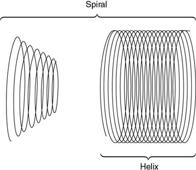
In another letter to the editors of AJR, Silverman et al. (1994) argued that the term helical CT “best describes this new CT technology.” Dr. Mark Bahn of the Mallinckrodt Institute of Radiology offered mathematical definitions to support this view. He pointed out that mathematical dictionaries (Baker, 1961; James & James, 1976) provide more technical definitions of these two terms: a spiral describes a curve on a plane surface; a helix describes a curve in 3D space.
In response, Kalender (1994a) submitted a letter (Appendix A) to the editors of Radiology to support use of the term spiral CT, which convinced the editors to accept either term for CT papers published in in their journal. This book uses both terms as synonyms, as suggested by Kalender (1994a).
Conventional slice-by-slice CT scanning
Scanning sequence
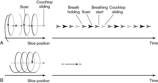
In conventional CT scanning, the x-ray tube rotates around the patient to collect data from a single slice of tissue, followed by table indexing so that the next contiguous slice can be scanned. This process is repeated until data from several contiguous slices have been collected. The scanning sequence for this type of data acquisition consists of four distinct steps (Fig. 12.2).
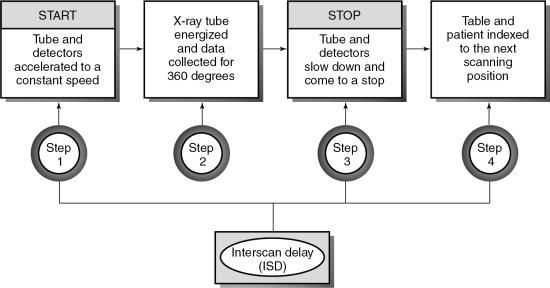
In the first step, the x-ray tube must be accelerated to a constant speed of rotation. This means that the cables that supply power to the x-ray tube must be long enough to allow for the full 360-degree rotation. During this rotation (step 2), the x-ray tube produces x-rays that are transmitted through the patient to fall on the detectors, which measure the relative transmission values (data). At this particular point, the patient holds a breath, and data are collected from a specific axial slice. In step 3, the patient resumes breathing while the x-ray tube slows to a stop. In step 4, it is necessary to unwind the cable because of the 360-degree rotation and to move the patient and table so that the next contiguous slice can be scanned.
This four-step process is repeated until all the required contiguous axial slices have been scanned. The time it takes to accomplish steps 1, 3, and 4 is referred to as the interscan delay time (ISD).
Slices are usually collected in groups while the patient holds a breath, with the ISD after each pair of slices. Between two groups of slices is an intergroup delay, and it is at this point that the patient breathes. Additionally, the scan rate is expressed as the following ratio:
If the study requires more slices, its duration would have to be increased. This requirement places an additional burden on the patient to remain still to ensure that images obtained are free of motion artifacts.
Limitations
The limitations imposed by slice-by-slice sequential CT scanning include the following:
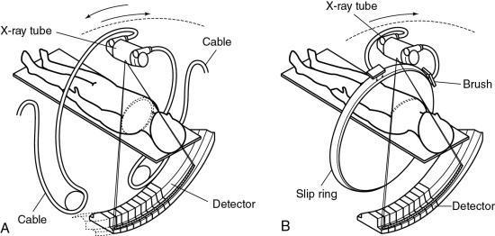
- 1. Longer examination times because of the stop–start action necessary for patient breathing, table indexing, and cable unwinding. This gives rise to the ISD. The cable wraparound and unwinding is shown in Fig. 12.3A. This wraparound results from the fixed length of the high-voltage cable, which follows the x-ray tube as it rotates through 360 degrees around the patient. The cable is unwound during the imaging of the next slice. In Fig. 12.3B, the cable wraparound process is eliminated through the use of slip-ring technology, which allows the x-ray tube to rotate continuously as the patient moves continuously through the gantry. This is spiral/helical CT scanning.
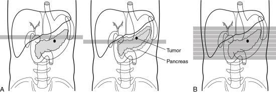
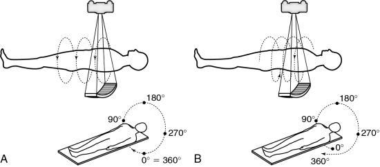
- 2. Certain portions of the anatomy are omitted because the patient respiration phase may not always be consistent between scans (Fig. 12.4). For example, it has been reported that lesions in the liver smaller than 1 cm may be missed because of inconsistent levels of inspiration. This omission of anatomy is often referred to as slice-to-slice misregistration.
- 3. Inaccurate generation of 3D images and multiplanar reformatted images are attributed to the inconsistent levels of inspiration from scan to scan. The result is the appearance of “steplike” contours in 3D images. Fig. 12.5 illustrates production of the stairstep artifact and its elimination with spiral/helical CT.
- 4. Only a few slices are scanned during maximum contrast enhancement when the contrast enhancement technique is used. These problems may be overcome if the scan rate is increased and the ISD is eliminated, both of which are technologically feasible. The scan time can be increased by decreasing the time to accomplish the four steps shown in Fig. 12.2. The ISD can be eliminated by having the tube (and detector) rotate continuously around the patient (instead of the start–stop action characteristic of slice-by-slice sequential CT scanning) while simultaneously translating the patient through the gantry aperture at a faster speed. Data are acquired during the patient translation.
This chapter concentrates on methods to remove the ISD with the goal of acquiring the data continuously rather than in slices. This technique is only possible with continuous rotation scanners based on slip-ring technology.
Principles of SSCT scanners
The introduction of CT scanners that can scan rapidly with scan times shorter than 1 second has led to the development of the SSCT scanner. The overall goal of this scanner is to increase the volume coverage speed compared with that of the conventional CT scanner.
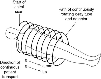
To do this efficiently requires that the x-ray tube rotate continuously around the patient while the patient moves through the gantry aperture during the scanning to cover an entire volume of tissue (compared with a single-slice characteristic of conventional CT scanners). Rotation of the x-ray tube coupled with patient translation through the gantry aperture traces an x-ray beam path with respect to the patient (Fig. 12.6). The path geometry describes a spiral or helical winding and therefore has been referred to as spiral/helical CT. Other terms considered synonymous are spiral volume CT and helical volumetric CT.
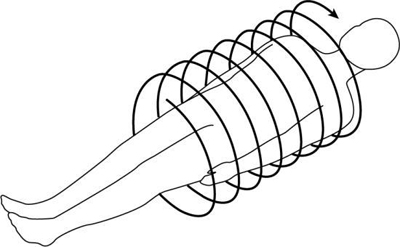
Because a 1D detector array is used, only a single slice is acquired during one rotation of the tube. Because there are several rotations per required length of anatomy imaged (volume of tissue scanned), several slices of tissue and corresponding images can be computer generated for the volume of the anatomy scanned during a single breath-hold.
Requirements for volume scanning
Because the data in spiral/helical CT are collected in volumes rather than slices, the following requirements must be met:
- 1. Continuously rotating scanner based on slip-ring technology
- 2. Continuous couch movement
- 3. Increase in loadability of the x-ray tube, capable of delivering at least 200 mA per revolution continuously throughout the time it takes to scan the volume of tissue
- 4. Increased cooling capacity of the x-ray tube
- 5. Spiral/helical weighting algorithm
- 6. Mass memory buffer to store the vast amount of data collected
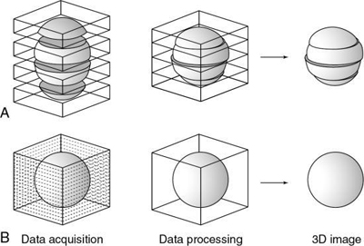
Data acquisition
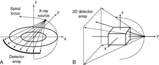
The first step in volume scanning is data acquisition (Fig. 12.7). The x-ray tube traces a spiral/helical path with a radius equal to the distance from the focal spot to the center of rotation. This results in an entire volume of tissue being scanned during a single breath-hold compared with slice-by-slice imaging (Fig. 12.8).
Transporting the patient through the gantry during the scanning process is referred to as the table feed speed in millimeters per second (Fukuda et al., 2014). Very fast table feed (mm/rotation) leads to image degradation caused by motion artifacts or may cause the patient to feel motion sickness. The table feed speed varies from vendor to vendor and can be categorized as low, intermediate, and high speeds (Fukuda et al., 2014).
Several problems can result from data acquisition with spiral/helical beam geometry:
- 1. There is no defined slice, and thus localization of a particular slice is difficult.
- 2. The geometry of the slice volume is different for spiral/helical scans compared with conventional CT scans (Fig. 12.9). Fig. 12.10 explains the origin of the slice volume shown in Fig. 12.9B. In conventional slice-by-slice CT, the tube rotates around the patient for 360 degrees to collect a complete set of data in planar geometry for each individual slice shown in Fig. 12.9A. This dataset is said to be consistent; that is, it is collected from one slice or plane. In spiral/helical volume CT scanning, the x-ray tube rotates continuously as the patient moves through the gantry continuously as well. In this situation, data are now collected in nonplanar geometry, resulting in the diagram shown in Fig. 12.9B. These data are collected from different regions of the volume and not through a particular plane.
- 3. The effective slice thickness increases because it is influenced by the width of the fan beam and the speed of the table.
- 4. Because of the absence of a defined slice, the projection data are inconsistent (consistent projection data are needed to satisfy the standard reconstruction process).
- 5. When inconsistent projection data are used with the standard reconstruction process, streak artifacts akin to motion artifacts are clearly apparent on the image.
These problems can be solved through the use of special postprocessing techniques. One such method involves a “dedicated reconstruction algorithm that synthesizes raw data representing a perfectly planar slice from the original spiral data by interpolation” (Kalender, 1995). Interpolation is a mathematical technique in which an unknown value can be estimated given two known values on either side (see Chapter 5). Interpolation and extrapolation are illustrated in Fig. 12.11.
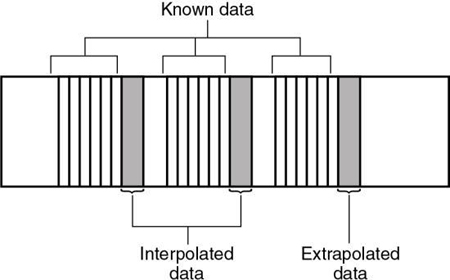
Image reconstruction
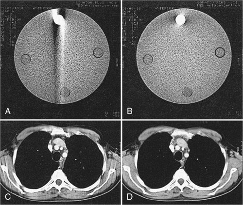
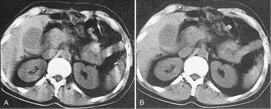
Inconsistent data obtained from 360-degree spiral/helical scan rotation are used directly in the image reconstruction process. Motion artifacts are apparent as shown in Fig. 12.12, for phantom images, and in Fig. 12.13, for patient images.
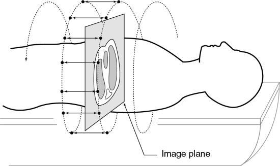
To eliminate these motion artifacts arising from the continuous movement of the patient during scanning, two steps are needed:
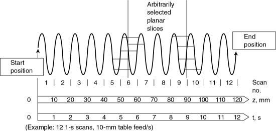
- 1. Calculation (using interpolation) of a planar dataset from the tissue volume dataset for every image (Fig. 12.14). The planar dataset (the image plane in Fig. 12.14) approximates the transverse axial section as with conventional CT. Within the volume scanned, a slice can be selected anywhere between the start and end positions in addition to the spacing and the number of slices (Fig. 12.15).
- 2. Reconstruction of images similar to conventional CT by use of the filtered back-projection algorithm. The results of these two processes are free of blurring as shown in Fig. 12.13B.
A number of interpolation algorithms are used to produce the planar dataset, and linear interpolation (LI) represents the “simplest approach” (Kalender, 1995). Two interpolation algorithms for SSCT are the 360-degree LI algorithm and the 180-degree LI algorithm.
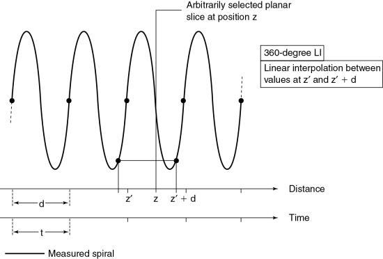
360-degree linear interpolation algorithm
The 360-degree LI algorithm was the interpolation algorithm used during the initial development of spiral/helical CT scanners (Fig. 12.16). The basis for this algorithm is illustrated in Fig. 12.16. The planar slice is interpolated by use of data points measured 360 degrees apart. The fundamental problem with the 360-degree LI algorithm is related to the image quality of the planar slice. This algorithm broadens the slice sensitivity profile (SSP) and hence degrades image quality. To overcome this problem, the 180-degree LI algorithm was introduced.
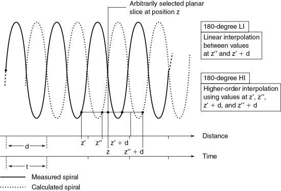
180-degree linear interpolation algorithm
The 180-degree LI algorithm improves the image quality of the 360-degree LI algorithm by using points that are closer to the planar slice to be interpolated (Fig. 12.17). The basic difference between the 360-degree and the 180-degree LI algorithms is that a second spiral (the dotted line in Fig. 12.17) is calculated from the measured spiral/helical dataset and is offset by 180 degrees. In this situation, the planar slice can then be interpolated with use of data points that are closer to it compared with the 360-degree LI algorithm. This process improves on the SSP and therefore enhances image quality.
In addition to these algorithms, Kalender (1995) stated that “higher-order nonlinear interpolation algorithms can be implemented. While they preserve the shape of the sensitivity profiles even better, their influence on noise and image quality is not easy to predict and control. On a given scanner, the exact algorithm and above all its implementation, which may have significant influence on image quality and artifact behavior, are not documented as they are considered confidential by the manufacturers in most cases.”
These algorithms are not within the scope of this book. The reader should refer to Kalender (2005) for a further description of nonlinear interpolation algorithms.
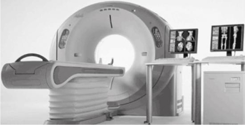
Instrumentation
Spiral/helical CT scanners (SSCT or MSCT; Fig. 12.18) are not different in external appearance from conventional CT scanners. However, there are significant differences in several major equipment components.
Equipment components
A block diagram of the major equipment components of a spiral/helical CT scanner is shown in Fig. 12.19. The most noteworthy feature is the use of slip rings to connect the stationary and rotating parts of the scanner.
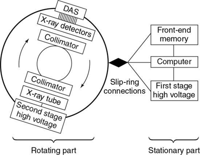
The rotating part of the system consists of the x-ray tube, high-voltage generator, detectors, and detector electronics (DAS). The stationary part consists of the front-end memory and computer and the first-stage high-voltage component.
The x-ray tube and detectors rotate continuously during data collection because the cable wraparound problem has been eliminated by slip-ring technology. Because large amounts of projection data are collected very quickly, increased storage is needed. This is accommodated by the front-end memory, fast solid state, and magnetic disk storage.
In spiral/helical CT scanners (SSCT and MSCT) the x-ray tube is energized for longer periods of time compared with conventional CT tubes. This characteristic requires x-ray tubes that are physically larger than conventional x-ray tubes and have heat storage capacities greater than 3 million heat units (MHUs) and anode cooling rates of 1 MHU/min (Bushong, 2017).
X-ray detectors for single-slice spiral/helical CT scanning are 1D arrays and should be solid state because their overall efficiency is greater than gas ionization detectors.
The high-voltage generator for spiral/helical CT scanners is a high-frequency generator with a high-power output. The high-voltage generator is mounted on the rotating frame of the CT gantry and positioned close to the x-ray tube (see Fig. 12.19). X-ray tubes operate at high voltages (about 80 to 140 peak kilovolts) to produce x-rays with the intensity needed for CT scanning. At such high voltages, arcing between the brushes and rings of the gantry may occur during scanning. To solve this problem, one approach is to divide the power supply into a first stage on the stationary part of the scanner, where the voltage is increased to an intermediate level, and a second stage on the rotating part of the scanner, where the voltage is increased to the required high voltages needed for x-ray production and finally rectified to direct current potential (see Fig. 12.19; Napel, 1995). Another approach passes a low voltage across the brushes to the slip rings, the high-voltage generator, and then the x-ray tube. In both designs, only a low to intermediate voltage is applied to the brush/slip-ring interface, thus decreasing the chances of arcing.
Slip-ring technology
One of the major technical factors that contribute to the success of spiral/helical CT scanning is slip-ring technology (see Fig. 12.19). The purpose of the slip ring is to allow the x-ray tube and detectors (in third-generation CT systems; Fig. 12.19) to rotate continuously so that a volume of the patient, rather than one slice, can be scanned very quickly in a single breath-hold. The slip rings also eliminate the long, high-tension cables to the x-ray tube used in conventional start–stop CT scanners. As the x-ray tube rotates continuously, the patient also moves continuously through the gantry aperture so that data can be acquired from a volume of tissue.
The technical aspects of using slip rings for data acquisition are described in Chapter 4. These include the design and power supply to the rings and a comparison of low-voltage and high-voltage slip-ring CT scanners in terms of the high voltage supplied to the x-ray tube.
Basic scan parameters
Several scan parameters for SSCT and MSCT are the same as for conventional CT; however, there are a few parameters and a set of terms associated only with spiral/helical CT. Typical parameters include spiral/helical scan time, table feed per 360-degree rotation, table speed, number of revolutions, scan range or volume coverage, z-axis (the axis of rotation of the scanner or the longitudinal axis of the patient), collimation, and the reconstruction increment and z-interpolation (“calculation of planar attenuation data for desired table position interpolation between data points measured for the same projection angle at neighboring z-axis positions [synonyms: slice interpolation, section interpolation, z-axis interpolation]”) algorithms (Kalender, 1995). It is beyond the scope of this chapter to describe all of these parameters; however, important ones such as the pitch, beam geometry, collimation, and slice thickness will be described later here.
Limitations of SSCT scanners
Ever since its introduction in 1990, single-slice volume CT has been used successfully in many body CT imaging applications in which speed and volume coverage are important. Volume coverage and speed can be increased by using higher pitch ratios; however, higher pitch ratios in single-slice volume CT scanning degrade image quality (z-axis resolution) and produce image artifacts. In SSCT, the volume coverage speed is limited, especially in clinical applications that demand large-volume scanning with critical timing requirements and optimum image quality (z-axis resolution and low image artifacts), such as CT angiography with 3D, multiplanar reformatting or reconstruction (MPR), and maximum intensity projection (MIP) techniques (Hu, 1999). Single-slice volume CT is based on the use of a single row of detectors (1D detector array). Because the x-ray beam is highly collimated to the size of the detector array, only a small percentage of x-rays emitted by the tube is used in the imaging process. This situation is described as poor geometric efficiency. Also, SSCT uses the 360-degree linear interpolation algorithm (LIA) and the 180-degree LIA to improve the problems imposed by the 360-degree LIA, such as poor image quality and artifact production. However, the 180-degree LIA produces more noise while preserving the detail (slice sensitivity and spatial resolution). Additionally, the time duration for covering defined volumes in SSCT (several seconds) is limited by several factors, such as the ability of some patients, particularly those who are critically ill, to maintain a single breath-hold during volume scanning and the heat loading of the x-ray tube.
SSCT is also limited in its ability to meet the needs of time-critical clinical examinations such as multiphase organ dynamic studies and CT angiography, in which both arterial and venous phases are extremely important, with smaller amounts of contrast media. The use of higher pitch ratios to solve these problems degrades the slice sensitivity profile (detail). Therefore, other methods are needed to overcome these limitations to improve the performance of SSCT in terms of better use of the x-ray output (improved geometric efficiency) and scan parameters affecting image quality and volume coverage.
MSCT offers “substantial improvement of the volume coverage speed performance” (Hu, 1999). This means that MSCT provides faster scanning and higher resolution for a number of clinical applications (Taguchi & Aradate, 1998). One of the most conspicuous differences between MSCT and SSCT is that the former uses a multiple row of detectors (2D detector array), whereas the latter uses a single row of detectors (1D detector array), as is clearly illustrated in Fig. 12.20.
Evolution of multislice CT scanners
Terminology
Several terms are used in the literature to refer to MSCT, including multisection CT, MDCT, multidetector row CT, and multichannel CT (Cody & Mahesh, 2007; Douglas-Akinwande et al., 2006). Each of these terms appears to focus on a particular outcome characteristic. For example, although the terms multislice and multisection focus on images, the terms multidetector and multidetector row focus on the detectors used during the scanning. Finally, the term multichannel refers to the function of the DAS. In this book, the term multislice CT (MSCT) will be used because it has become commonplace not only in the literature but also in clinical practice (Dowsett, 2006; Kachelriess et al., 2006; Kalender, 2005).
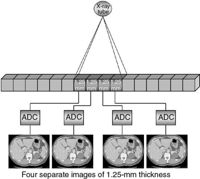
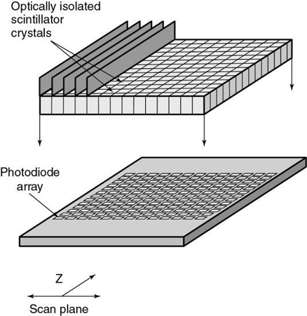
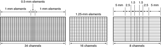
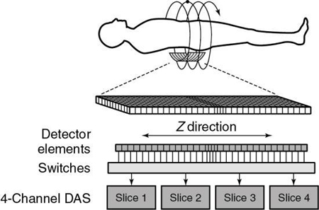
A CT detector consists of basically two major components: a radiation sensor coupled to suitable electronics, such as photodiodes, and analog-to-digital converters (ADCs; see Chapter 4). Although the radiation sensors convert x-ray photons to light, the photodiodes convert the light into electrical current (signal) that must be digitized before it is sent to a digital computer for processing. The electronics are carefully configured to the sensor elements (cells) of the CT detector and represent the data acquisition channels. As seen in Fig. 12.21, the detector consists of 16 elements or cells, each 1.25 mm in size, and the x-ray beam is collimated to fall on four of these cells. Therefore, four signals are collected per gantry rotation from each of the four cells and sent to the four ADCs to produce four slices, each 1.25 mm thick. For eight 1.25-mm thick slices, the x-ray beam would fall on eight detector elements. For four 2.5-mm thick slices, the beam would be collimated to fall on eight detector elements, where two 1.25-mm elements would be combined to produce a 2.5-mm thick slice, and so on. This electronic combination (or binning) of detector elements is described in more detail later in this chapter.
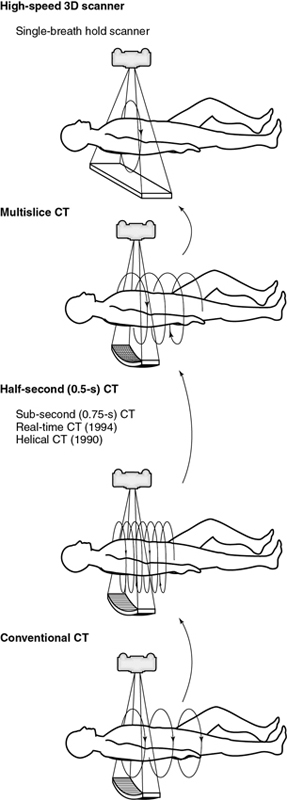
The evolution of MSCT technology is outlined in Fig. 12.22. Its overall goal is to improve volume coverage speed performance; therefore, scanning is at higher speeds with higher pitch ratios to cover large volumes with equivalent image quality compared with single-slice volume CT scanners introduced in the 1990s. The 256-slice CT scanner was introduced by the Toshiba Corporation Medical Systems Division as a prototype high-speed 3D CT scanner for imaging the entire heart in one complete rotation. The high-speed 3D scanner will use larger area detectors to scan larger volumes at high speeds and subsequently display all images in 3D. Finally, in 2008, Toshiba Medical Systems introduced a new 320-slice CT scanner. These two scanners will be described briefly later in this chapter.
Sub-second scanners
Scanning time continues to decrease from the 5 minutes needed by the original EMI scanner to as low as 0.5 second at present. The engineering barriers to be overcome in reaching this gantry speed are formidable. The acceleration on gantry components such as the tube and generator can reach 13 gravities (Gs), considerably more than experienced by the space shuttle at lift off. Some interesting technological developments have accompanied the design of these high-speed CT systems.
To prevent anode movement under the stress of sub-second acceleration, new x-ray tubes have the anode mounted on a shaft that extends along the tube, providing support on both sides of the anode. This design has distinct advantages over the traditional method of supporting a massive anode from the rear only. Other innovative developments in tube design for CT include grounded anodes and a technique to reduce off-focal x rays. Virtually all medical x-ray tubes have applied the potential difference equally between cathode and anode so that the cathode can be at 75 kV while the anode is at 75 kV. This requires a substantial gap between the anode and the tube housing to reduce the possibility of arcs. With all the voltage placed on the cathode and the anode at ground potential, the tube housing can be brought into close proximity to the anode, which facilitates heat transfer and markedly improves anode cooling rate. Recoil electrons, which normally are re-attracted to the anode and generate off-focal x rays, can now be collected on a special collimator located near the anode. This eliminates off-focal x rays that can reduce image quality and reduces the anode heat loading by about 30%, thereby reducing tube cooling delays during routine scanning.
The clinical benefits of sub-second scanning include reduced motion artifacts and greater scan coverage. Patient movement during CT scanning, whether by cardiac motion, breathing, or peristalsis, may cause artifacts because filtered back-projection reconstruction combines all the views acquired during the scan rotation to cancel artifacts. Movement of any object in the field of view (FOV) during gantry rotation prevents accurate elimination of artifacts with consequent loss of image quality. If the moving object has notably high or low contrast, such as bone, calculi, or air, the artifacts are particularly noticeable. Unfortunately, the left ventricle and pulmonary vessels near the heart move so quickly that scans would have to be completed in less than 20 ms to 25 ms to completely eliminate all blurring. This is a far shorter time than is possible with conventional CT scanners and is even difficult for electron-beam CTs, which are extremely fast. Even so, the half-second scanners, which can acquire “partial” (i.e., less than 360-degree rotation) images in 250 ms to 320 ms, have made it feasible to obtain considerably better images of the heart and chest than is possible with a 1-second system. An example is the ability of these scanners to use gated reconstruction, in which the raw scan data for image reconstruction can be selected on the basis of the patient’s electrocardiogram (ECG). Reconstruction of a gated “partial” image during cardiac diastole, when the heart is relatively quiescent, can show fairly sharp ventricular borders and calcium in the coronary arteries.
Prospective gating can also be used in which the patient’s ECG triggers the actual scan acquisition. This is a relatively simple technique, although it is not applicable to spiral/helical scanning.
A less dramatic but very practical benefit of sub-second scan times is the increased spiral/helical coverage that can become available. For the same pitch and scan duration, a half-second scanner will cover twice the anatomy that can be acquired with a 1-second scanner.
Alternatively, the half-second scanner could cover the same area by using 50% of the slice thickness, which improves z-axis resolution and leads to better image quality in 3D and multiplanar reconstructions. Clinical applications, such as CT angiography (CTA), can benefit from increased patient coverage without increasing pitch. This assumes that the system generator is able to produce enough power to accommodate the faster scans. For example, a 250-mA image of the abdomen requires a tube current of 500 mA in a half-second scanner.
Dual-slice CT scanners
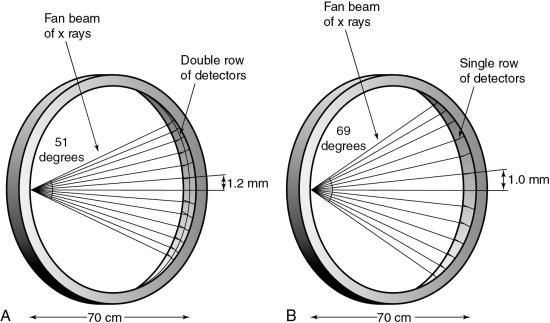
The history of scanning more than one slice at a time (actually two-slice scanners) dates back to one of the early EMI (London, United Kingdom) CT scanners, which became available in 1972, and the Siemens SIRETOM (Siemens Medical Solutions, Germany, personal communications) CT scanner, which appeared in 1974. These scanners used two detectors based on the translate/rotate method of data collection over 180 degrees. The next major step to MSCT scanning appeared in 1993, with the introduction of the first dual-slice volume CT scanner, the Elscint CT-TWIN (Elscint, Hackensack, NJ, personal communications). The most significant difference between the dual-slice volume CT scanner and its single-slice counterpart is shown in Fig. 12.23. As can be seen, the dual scanner slice geometry is based on a fan beam of x rays falling on two rows of detectors (see Fig. 12.23A) instead of one row of detectors, characteristic of the SSCT scanner beam geometry (see Fig. 12.23B).
The dual-slice whole-body fan-beam CT scanner offers improved volume coverage speed performance compared with the single-slice volume CT scanner, reducing the scan time by 50% while maintaining image quality for the same scanned volume.
Multislice CT scanners
The dual-slice whole-body fan-beam CT technology paved the way for the development of other MSCT scanners. These scanners were introduced at the 1998 meeting of the RSNA in Chicago. They are based on spiral/helical scanning using multiple detector rows ranging between 8, 16, 32, 40, 64, (Kohl, 2006a), 256 (Mori et al, 2006a), 320, and more recently 640 (Lu et al., 2019) depending on the manufacturer. The 256-slice prototype scanner paved the way for the 320-slice dynamic volume CT scanner. This scanner is highlighted later in the chapter.
The overall goal of the MSCT scanner is to improve the volume coverage speed performance of both single-slice and dual-slice CT scanners. For example, an MSCT scanner with N-detector rows (N slices) will be N times faster than its single-row (one slice) counterpart. Thus, MSCT opens new avenues and opportunities to improve the quality of care afforded to patients because it now offers a wide range of new clinical applications afforded by recent technological developments.
Physical principles
Although the fundamental physics and flow of data are the same as conventional and spiral/helical CT scanners, MSCT scanners introduce several new concepts relating to detector technology, the geometry of data acquisition, slice selection, and multislice image reconstruction algorithms.
Data acquisition
Data acquisition is one of two mechanisms that affect image quality in CT (the other is image reconstruction). This section examines data acquisition in MSCT with respect to beam geometry and basic parameters such as collimation, slice thickness, and pitch; but first a brief review of data acquisition in SSCT is in order.
SSCT
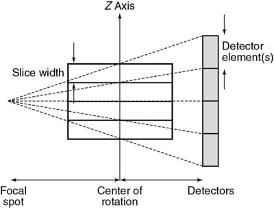
The basic data acquisition geometry for SSCT is shown in Fig. 12.24. This is a third-generation scheme in which the x-ray tube is coupled to a single-row detector array positioned in the z-axis.
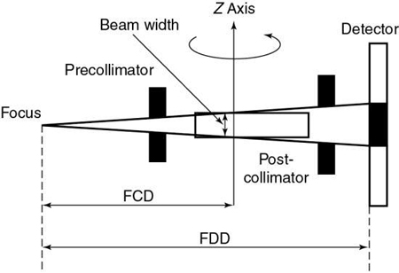
Collimation.
The x-ray beam collimation system is designed to ensure a constant beam width because the precollimator and postcollimator widths are equal. The beam may or may not be collimated at the detector array. The width of the precollimator defines the slice thickness (z-axis resolution or spatial resolution) and affects the volume coverage speed performance. Although thin collimation results in better resolution and takes longer to scan a specified volume, wide collimation results in less resolution but provides better volume coverage speed. The beam width (BW) is measured in the z-axis at the center of rotation for a single-row detector array, and it is defined by the precollimator width, which determines the thickness for a single slice. A collimator width of 8 mm falling on a 1D detector array will provide a slice thickness of 8 mm.
Beam geometry.
The x-ray beam geometry for SSCT describes a small fan (see Fig. 12.24) and is referred to as a parallel fan-beam geometry.
Pitch.
The pitch for SSCT is defined as the ratio of the distance the table travels per gantry rotation to the BW or precollimator width.
Slice thickness.
In SSCT, the thickness of the slice is determined by the pitch and the width of the precollimator (which also defines the BW) at the center of rotation (see Fig. 12.24).
MSCT
The data acquisition geometry for MSCT is shown in Fig. 12.25. Perhaps the most conspicuous difference between the data acquisition geometry in Figs 12.24 and 12.25 is the multirow detector array (specifically 4) coupled to the x-ray tube to describe a third-generation geometry (Fig. 12.25A). Unique features of multislice data acquisition are the 2D detector array, collimation, beam geometry, and pitch.
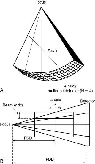
Collimation.
The fundamental collimation scheme is shown in Fig. 12.20B. The beam is collimated by a precollimator to fall on the entire multirow detector array. The BW is still defined in the z-axis at the center of rotation but now is for a four-row multislice detector array, as shown in Fig. 12.25B. This width will be for four slices and is prescribed by the precollimator. A precollimator width of 8 mm that falls on a four-row multislice detector array will produce four slices, each with a thickness of 2 mm (i.e., 8 mm—the total beam width in the z-axis at the center of rotation divided by 4). This is unlike the single-slice counterpart, which provides a slice thickness of 8 mm with its 8-mm-wide precollimator. In addition, the four slices are a result of the division of the total x-ray beam into multiple beams, depending on the number of arrays in the 2D detector system. These multiple beams are the result of the detector row collimation or the detector row aperture.
Fig. 12.26 is a side view of an MSCT scanner beam from the x-ray tube to the detectors. D is the width of the x-ray beam collimator and is measured at the axis of rotation, N is the number of detector rows, and d represents the detector row collimation. Hu (1999) explained that, if the gaps between the adjacent detector rows are small and can be ignored, the detector row spacing is equal to the detector row collimation (d). The detector row collimation d and the x-ray beam collimation D have the following relationship:
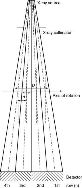

where N is the number of detector rows. In SSCT, the detector row collimation equals and is interchangeable with the x-ray beam collimation. “In multislice CT, the detector row collimation is only 1/N of the x-ray beam collimation.” This makes it possible “to simultaneously achieve high volume coverage speed and high z axis resolution. In general, the larger the number of detector rows N, the better the volume coverage speed performance” (Hu, 1999).
For example, if the x-ray prepatient collimation width (x-ray beam collimation) is 20 mm and the scanner has a four-row detector array, the detector row collimation is as follows:

in which d is the detector row collimation, N is the number of detector rows, and D is the x-ray beam collimator width (20/4 = 5 mm).
Alternatively,
As the beam width increases in the z direction to cover the number of rows in the 2D detector system, the amount of scattered radiation increases because a wide area of the patient is scanned. To minimize scattered radiation, antiscatter collimation may be used at the detector array (postcollimation). One such scheme is shown in Fig. 12.27. Another scheme is illustrated later.
Beam geometry.
As the number of detector rows in a multirow detector array increases, the beam becomes wider to cover the 2D detector array (Fig. 12.28; see also Fig. 12.26). The beam must cover the length of the detector array. This coverage is influenced by the fan angle of the beam, in which a wider fan angle will cover a longer detector array. The beam must also cover the width of the detector array, which is defined by the number of rows in the detector array. A larger number of rows will result in a wider beam (large cone beam) in the z-axis direction.
A cone-beam geometry produces more beam divergence along the z-axis compared with fan-beam geometry. For this reason, increasing the number of detector rows in MSCT creates a need for a different approach to the interpolation process (compared with single-slice spiral/helical interpolation) because the rays that contribute to the imaging process are more oblique. In addition, the number of detector rows plays an important role in slice thickness selection and volume coverage.
Pitch - international electrotechnical commission definition
The pitch is a term associated with a fastener, and it is actually the distance between the turns on the fastener. In spiral/helical CT, the pitch is defined as the distance (in mm) that the CT table moves during one revolution of the x-ray tube. The pitch is used to calculate the pitch ratio, which is a ratio of the pitch to the slice thickness or beam collimation. The pitch ratio is as follows:
When the distance the table travels during one complete revolution of the x-ray tube equals the slice thickness or beam collimation, the pitch ratio (simply referred to as pitch in the remainder of this text) is 1:1, or simply 1. A pitch of 1 results in the best image quality in spiral/helical CT scanning. The pitch can be increased to increase volume coverage and speed up the scanning process. Pitch is of particular significance because it affects image quality and patient dose and also plays a role in the overall outcome of the clinical examination. A pitch of less than 1 is effectively the same as overlapping slices and imparts a high dose. Conversely, pitches of greater than 1 result in reduced patient dose.
The introduction of multislice detectors resulted in a re-evaluation of the definition of pitch, and in the past, the definition was somewhat varied and controversial. For a discussion of such controversy, beginning in the 1990s, the interested reader should refer to Hu (1999), He (personal communication, 1999), Taguchi and Aradate (1998), and Kalender (2005).
In 1999, the International Electrotechnical Commission (IEC) introduced a definition of pitch, which is stated in the IEC document 60601 regulation for CT, as a means of addressing the variations in definitions offered by different manufacturers (IEC, 1999). The IEC recommends the following:
The total collimation, on the other hand, is equal to the number of slices (M) times the collimated slice thickness (S). Algebraically, the pitch can now be expressed as follows:
For a patient dose comparable to current single-slice scanners at a pitch of 1, a four-slice scanner would require a beam pitch of 1 or a slice pitch of 4. As an example, selection of 4 × 5-mm slices with a table speed of 20 mm per rotation should result in approximately the same patient dose as from a single-slice scanner operated with a 5-mm slice at 5 mm per rotation table speed. Whether this is true in practice depends on the collimator design of the specific scanner.
Slice thickness
In MSCT, the slice thickness is determined by the BW (see Fig. 12.25), the pitch, and other factors such as the shape and width of the reconstruction filter in the z-axis. The details of slice thickness selection for MSCT scanners are described later in this chapter.
Image reconstruction
In conventional step-and-shoot CT (conventional CT), a fan-beam geometry and a single-row detector array are used in the data acquisition process, and all rays pass through the image plane (planar section), the slice of interest. With this condition, a fan-beam reconstruction algorithm, specifically, the filtered back-projection algorithm, is used for image reconstruction.
Single-slice spiral/helical reconstruction
In SSCT scanners, the fan-beam geometry is maintained and a single-row detector array is used in the data acquisition process. In conventional CT, the patient is stationary during scanning, whereas in SSCT the patient is moving continuously through the gantry aperture during a 360-degree rotation of the x-ray tube and detectors. In this case, all rays do not pass through the image plane. A fan-beam geometry is used, so the fan-beam reconstruction algorithm used in conventional CT is used for image reconstruction. During data acquisition, the fan beam traces a spiral/helical path around the patient, as shown in Fig. 12.29. Because all rays do not pass through the image plane (planar section), SSCT requires an additional step of first calculating a planar section. This is done by interpolation, using data points on either side of the section.
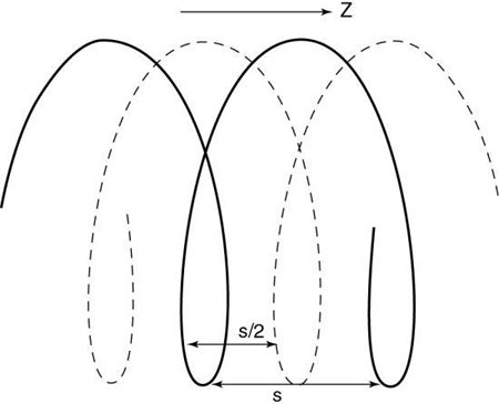
The first interpolation algorithm used was 360-degree LI, in which the distance between the two data points used in the interpolation was represented by s in Fig. 12.29. In an effort to improve the image quality resulting from the 360-degree LI, a different algorithm was developed on the basis of the mathematical fact that a CT view from a specific angle contains the same information as a view in the opposite direction (at 180 degrees). The 180-degree view, when flipped and used for interpolated reconstruction, is referred to as complementary data, as opposed to the direct, measured data. With a 180-degree LI, data points are now closer to the image plane. The distance between the two points used for interpolation is now s/2. This equation involves calculation of a complementary dataset (dashed lines) using the direct fan-beam dataset or measurements (solid lines). The distance between the two points used for interpolation is referred to as the z-gap (Hu, 1999). The z-gap affects image quality so that the smaller the z-gap, the better the image quality. In single-slice spiral/helical CT, increased volume coverage can be achieved with increased pitch; however, as the pitch increases, image quality decreases because the z-gap becomes larger. This is one motivating factor for the development of MSCT.
Multislice reconstruction
One of the most conspicuous differences between SSCT and MSCT is that the latter uses a new detector technology in which the number of detector rows can vary from 4 to 320. These multiple detector rows result in a large 2D detector array. Because of this, a cone-beam geometry results instead of the fan-beam geometry characteristic of SSCT systems. Cone-beam geometry produces an increase in the beam divergence, which now poses a fundamental problem because all the rays do not pass through the image plane. Rays at the periphery of the beam lie outside the image plane. Approximate cone-beam reconstruction algorithms have been developed for solving this problem (Kudo & Saito, 1991); however, these particular algorithms demand extensive calculations (compared with fan-beam algorithms) and are not suitable for use in medical imaging.
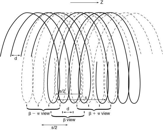
Special fan-beam reconstructions (Hu, 1999; Taguchi & Aradate, 1998) have been developed for MSCT in its present state. In deriving an algorithm for image reconstruction in MSCT, a logical first step is to extend the principles of 360-degree and 180-degree LI used in SSCT to MSCT. To examine this extension, consider Fig. 12.30, which shows the spiral/helical path of a four-row detector array used in MSCT. For a 360-degree LI, the distance between the two points used for interpolation of a planar section is s, the same distance as in Fig. 12.29 for SSCT. With a 180-degree LI, the distance of the data points is s/2 (distance between the solid and dashed lines of the same detector row). The z-gap is the same as for SSCT.
MSCT for up to four detector rows.
In MSCT, the z-gap is determined by the pitch (as in SSCT) and by the detector row spacing, d. “As the helical pitch varies, distinctively different z sampling patterns and therefore interlacing helix patterns may result in multislice helical CT” (Hu, 1999). This is illustrated in Fig. 12.31 for a four-row detector array for two different pitches. At a pitch of 2:1 (see Fig. 12.31A) the distance between the points used for interpolation, the z-gap, is d, “which is the same as the displacement from one solid helix to the next. This causes a high degree of overlap between different helices, generating highly redundant projection measurements at certain z-positions. Because of this high degree of redundancy (or inefficiency) in z-sampling, the overall z-sampling spacing (i.e., the z-gap of the interlacing helix pattern) is still d, not any better than its single-slice counterpart” (Hu, 1999).
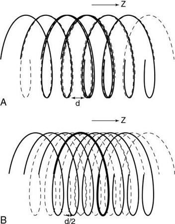
Increased pitch in MSCT from 2:1 to 3:1 (see Fig. 12.31B) results in a z-gap of d/2, a much shorter distance. In this case the volume coverage speed can be increased. In addition, because the z-gap is less as the pitch increases, better image quality results. Hu (1999) pointed out that “the volume coverage speed performance of the multislice scanner is substantially better than its single-slice counterpart, and so the selection of helical pitches is very critical to its performance. The pitch selection is determined by the consideration of the z-sampling efficiency and conventional factors such as volume coverage speed (which disfavors very low helical pitch); slice profile; and image artifacts, which disfavor very high helical pitch.” The preferred helical pitches are those that represent the preferred trade-offs for various applications.
Alternatively, Figs. 12.32 through 12.35 can be used to explain the problem and solution described previously. The unwound helical path for SSCT is shown in Fig. 12.32 for both direct and complementary data. The image plane is interpolated using two points from the direct data and the complementary data on either side of it (image plane). Extending the single-slice concept to the multislice case as shown in Fig. 12.33 results in a superimposition of the complementary and direct data for each of the detector rows in the four-row array. Note also that the z-gap is larger, and this results in image degradation. Additionally, the superimposition does not allow for efficient z-sampling. A pitch of 4 is not as preferable as a pitch of 2 because of the redundancy in the data sampling.
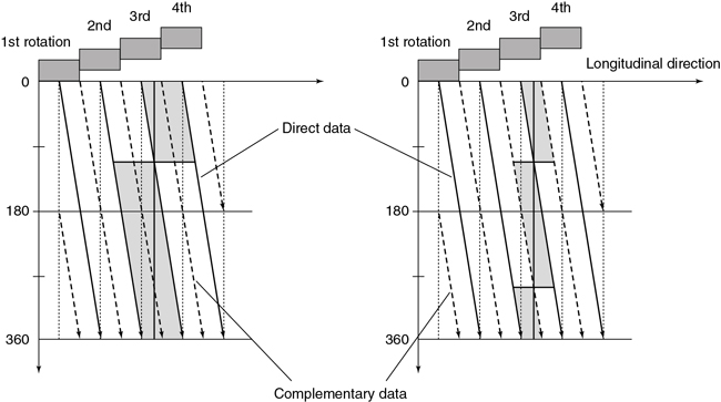
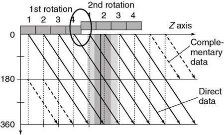
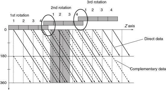
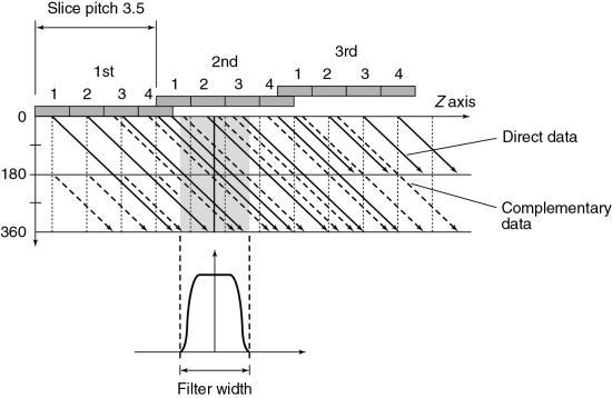
Fig. 12.34 provides a solution to the problem imposed by Fig. 12.33. By separating the direct and complementary data trails, efficient z-sampling can be achieved (Saito, 1998). Taguchi and Aradate (1998) referred to this as optimized sampling scan. Fig. 12.34 is with a pitch of 3.5 less than that of Fig. 12.33 (pitch of 4). These figures indicate that a slight compromise in helical pitch (just 0.5) produces amazing improvement in the data sampling pattern.
The detector design for MSCT allows the operator to select variable slice thicknesses on the basis of the requirements of the examination. The new algorithms for MSCT also allow for the reconstruction of these variable slice thicknesses. These new algorithms address problems (image quality degradation) arising from the increase in speed (hence volume coverage) of the patient moving through the gantry aperture when the pitch is increased. Additionally, these algorithms provide for the selection of the slice thicknesses that meet the needs of the examination.
In general, these algorithms are based on the following steps:
- 1. Spiral/helical scanning by interlaced sampling. In this step, smaller z-gaps are obtained by adjusting or selecting the pitch to separate the complementary data from the direct data.
- 2. Longitudinal interpolation by z-filtering. Another unique aspect of multislice data reconstruction involves averaging data in the z-axis direction. Interpolation of spiral/helical data is still needed, but the fact that the density of data points in this dimension is greater than with single-slice scanners is advantageous. One approach to image reconstruction uses a filter in the z-axis to select and weigh the data points to be used in the averaging (Taguchi & Aradate, 1998; Fig. 11-35). This method uses a filtering process in the longitudinal (z) direction. Assuming some range with a width called the filter width (FW) in the longitudinal (z) direction (see Fig. 12.35), all data sampled within that range are processed by weighted summation. The filter parameters (e.g., FW and shape) can control the spatial resolution in the longitudinal direction, the image noise, and the image quality. Again, pitch selection is flexible and should be carefully selected. A practical advantage of this technique is that the size and shape of the filter can be selected by the operator for more control over the effective slice thickness versus noise trade-off. As can be seen in Fig. 12.35, the selection of different FWs provides considerably more control over effective slice thickness than has generally been available with single-slice spiral/helical reconstruction. FW can also substantially affect image noise compared with conventional 180- or 360-degree LI.
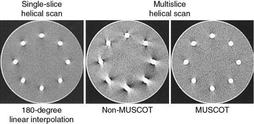
- 3. Fan-beam reconstruction. This algorithm can be used if the number of detector rows is small. Hu (1999) used multiple parallel fan beams to approximate the cone-beam geometry characteristic of MSCT. The algorithm used by Taguchi and Aradate (1998) is also based on a fan-beam method. Additionally, Saito (1998) labeled the algorithm multislice cone-beam tomography reconstruction method (MUSCOT). The effect of MUSCOT on image quality is shown in Fig. 12.36. Compared with SSCT (180-degree LI), MUSCOT provides good image quality “at a scanning speed that is about three times faster than that for single-slice CT” (Taguchi & Aradate, 1998).
MSCT for 16 or more detector rows.
The previous description lends itself to MSCT scanners with up to four detector rows. These scanners use a 2D detector array in which the x-ray beam is now opened in two dimensions to cover the entire detector array. The divergence of the beam describes a cone beam rather than a fan beam, and therefore the scanning geometry is now referred to as a cone beam. The nature and problems of using a cone beam with algorithms designed for fan-beam CT scanning geometries are outlined in Chapter 5. One of the problems, for example, is related to cone-beam artifacts (streaks, for example) that degrade image quality.
The algorithms for four-slice scanners described earlier ignore the cone-beam geometry in four-slice MSCT scanners because these algorithms assume that the measurement rays are parallel and perpendicular to the z-axis (longitudinal axis), a condition that satisfies the filtered back-projection (FBP) algorithm. Basically, the measurement rays for a planar dataset are obtained by interpolation with 360-degree LI or 180-degree LI algorithms similar to those for single-slice spiral/helical CT scanners (see Chapter 12), followed by the well-established and proven FBP algorithm.
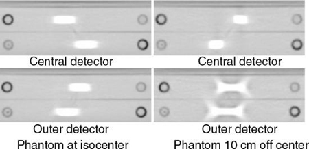
As the number of detector rows increases from 4 to 16 to 64 and beyond, the cone beam becomes larger and cone-beam artifacts become more pronounced, especially if the object imaged is not perfectly centered in the isocenter of the CT gantry (Fig. 12.37). The outer detectors receive more oblique rays compared with the central set of detectors. The effects of cone-beam geometries on image quality for these 16-slice and beyond MSCT scanners cannot be ignored. The cone-beam angle, for example, increases by up to 16, and previous interpolation algorithms are not useful for these large cone angles (Mather, 2005a). Therefore, cone-beam algorithms are needed to address these increasing cone-beam geometries and minimize cone-beam artifacts.
Cone-beam algorithms: A brief overview
Cone-beam algorithms fall into two classes: (1) exact algorithms and (2) approximate algorithms. Although exact algorithms for cone-beam data have not been successful in recent times (Kalender, 2005), they are also “computationally complex and difficult to implement” (Mather, 2005a). For these reasons, they are not described in this book. On the other hand, approximate cone-beam algorithms fall into two categories: 3D and 2D algorithms (Chen et al., 2003). Two such algorithms that have become commonplace in MSCT scanners are as follows:
Feldkamp-Davis-Kress algorithm
The fundamental basis of the FDK algorithm is illustrated in Fig. 12.38. As can be seen, the FDK algorithm simply is an extension of the 2D FBP for fan-beam geometry into a 3D FBP for cone-beam geometry (Chen et al., 2003; Kachelriess et al., 2006).
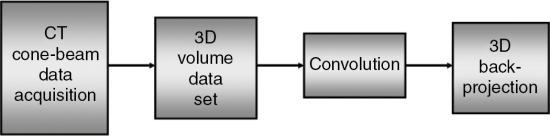
This algorithm is more extensive than the 2D FBP algorithm, and it is more commonplace for use with cone-beam CT scanners (Feldkamp et al., 1984; Hsieh et al., 2013). Although the 2D FBP algorithm filters the acquired data from 1D detectors, followed by a 2D fan-beam back-projection, the FDK algorithm filters the data acquired from 2D detectors (3D dataset) followed by a 3D cone-beam back-projection (Kalender, 2005).
There are several modifications of the FDK algorithm (referred to as Feldkamp-type algorithms) for use in MSCT scanners; however, the principles of these algorithms are beyond the scope of this book. Two examples of these algorithms in use on some MSCT scanners are the true cone-beam tomography Feldkamp-based algorithm developed by Toshiba Medical Systems, which can handle data from large cone angles, and the extended parallel back-projection algorithm developed by Siemens for scanners with more than 64 slices per rotation.
A basic problem with the Feldkamp-type algorithms is that they “cannot incorporate 2D back projection hardware already available in conventional medical CT systems” (Chen et al., 2003; Kachelriess et al., 2006). This problem, however, can be solved by 2D approximate algorithms.
Two-dimensional approximate algorithm
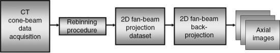
The main goal of the 2D approximate algorithms “is to provide an image quality close to that of a three-dimensional reconstruction algorithm using two-dimensional and back projection methods” (Chen et al., 2003). This principle is based on the notion of rebinning, a term used to describe the resorting of the 3D data collected from the cone-beam acquisition (geometry) to a set of 2D fan-beam projection data and, subsequently, use the conventional 2D FBP algorithm to reconstruct transaxial images, as illustrated in Fig. 12.39.
One early rebinning method was the single-slice rebinning (SSR) algorithm; however, it did not produce acceptable image quality for MSCT scanners with large cone angles. Therefore, other methods were developed to solve this problem by use of a technique called tilted plane reconstruction (TPR; Chen et al., 2003). The TPR method requires that the plane to be reconstructed is tilted (oblique) to fit the spiral/helical path of the x-ray beam to reduce cone-beam artifacts. One popular TPR algorithm is the ASSR algorithm used by General Electric (GE) Healthcare and by Siemens Medical Solutions.
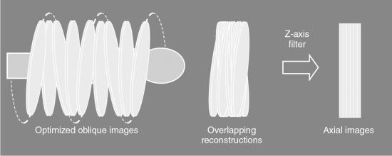
The fundamental steps of the ASSR algorithm, clearly illustrated in Fig. 12.40, are as follows:
- 1. The image planes to be reconstructed make use of 180-degree segments of the spiral/helical path of the x-ray beam to obtain optimized oblique images (semicircles) because they are tilted to fit the spiral path along the z-axis of the patient.
- 2. The measured cone-beam data are then rebinned (resorted) to produce a large number of overlapping, tilted reconstruction planes that can cover the entire volume of tissue imaged.
- 3. In the third step, z-axis reformation (z-axis filtering) is performed to produce axial images by using the conventional 2D reconstruction algorithm on the tilted planes.
- 4. Finally, step 3 produces an axial image dataset.
One of the fundamental problems with the ASSR algorithm is related to smaller pitch values. To solve this problem, the adaptive multiplane reconstruction (AMPR) algorithm was introduced. The AMPR algorithm is an extension of the ASSR algorithm and determines the z-axis resolution by allowing the free selection of pitch values and slice thickness (Flohr et al., 2005).
Another multislice cone-beam reconstruction algorithm somewhat related to the AMPR algorithm is the weighted hyperplane reconstruction algorithm. A hyperplane is a concept in geometry. In a 2D (x, y) space, a hyperplane is a line, whereas in a 3D (x, y, z) space, a hyperplane is an ordinary plane that separates the space into two halves (Oxford English Dictionary, 2008). Flohr et al. (2005) summarized this algorithm as follows:
“Similar to the AMPR, 3D reconstruction is split into a series of two-dimensional reconstructions. Instead of reconstruction of traditional transverse sections, convex hyperplanes are proposed as the region of reconstruction. The increasing spiral overlap with decreasing pitch is handled by introducing subsets of detector rows, which are sufficient to reconstruct an image at a given pitch value. At a pitch of 0.5625 with a 16-slice scanner the data collected by detector rows one to nine form a complete projection dataset. Similarly, projections from detector rows two to 10 can be used to reconstruct another image at the same z-axis position. Projections from detector rows three to 11 yield a third image and so on....The final image is based on a weighted average of the sub-images”
For a more detailed treatment of cone-beam algorithms, the interested reader should refer to Kalender (2005) and Flohr et al. (2005).
Instrumentation
In describing the instrumentation for MSCT systems, it is essential to focus on the major components responsible for data acquisition, image reconstruction, image display and manipulation, image processing, image storage, recording, and image transmission.
The flow of data in MSCT parallels that of conventional step-and-shoot CT and includes x-ray production and transmission through the patient and conversion of x-rays into electrical signals, which are subsequently converted into digital data for processing by a digital computer. Digital data in the computer are then converted into image data through image reconstruction, to be displayed on a monitor for viewing by an observer. However, the detector technology in MSCT is one of the most significant developments in the evolution of CT. Other components of significance are the DAS and the image reconstruction system for MSCT scanning.
The major equipment components for the MSCT imaging chain are the data acquisition components, patient couch or table, the computer system, and the operator console.
Data acquisition components
The MSCT gantry houses the x-ray generator, the x-ray tube, and detectors, as well as the detector electronics (DAS). MSCT scanners are based on the third-generation system design, in which the x-ray tube and detectors are coupled and rotate continuously during continuous patient translation through the gantry aperture. Such data collection strategy is possible through the use of slip-ring technology (see Chapter 4). Today contactless slip-ring technology has become available for use in CT scanners. For example, GE Healthcare (personal communication, 2014) reports that the Revolution EVO CT scanner, the next generation volume CT scanner, uses contactless slip ring “to transfer data to and from the rotating side of the gantry to the stationary side through RF technology at 40 Gbps. Induction based, brushless slip ring to reliably transfer high voltage power.”
These components (many of which are proprietary in nature and cannot be made publicly available) have improved through the years with the ultimate goal of improving imaging performance such as offering improved spatial resolution and generating images with low noise and reduced artifacts. It is a worthwhile exercise for the interested reader to explore the most recent CT manufacturer websites for state-of-the-art descriptions of the most recent technology as all new developments cannot be mentioned in this text.
X-ray generator
The x-ray generator is a compact, lightweight, high-frequency generator that provides a stable high voltage to the x-ray tube to ensure efficient performance such as high instantaneous power output from about 50 kW to 150 kW and high continuous power output. The power output (kW) of these generators varies depending on the manufacturer.
X-ray tube
The x-ray tube is a rotating-anode tube capable of high heat storage capacity with high anode and tube housing cooling rates. The x-ray beam is usually fan shaped and emanates from either a small or large focal spot. X-ray tubes for MSCTs provide tube voltages ranging from 70 kV to 150 kV in increments of 10 kV, and high tube current (mAs) variation, which is different depending on the manufacturer. In terms of evolution, x-ray tubes for CT scanning are always undergoing refinements to improve the performance output needed to image more sophisticated examinations that demand high x-ray output and short exposure times. For example, directly cooled (direct anode cooling) x-ray tubes are currently available from Philips and Siemens. See Chapter 4 for a more detailed description of x-ray tubes, including the most recent design for use with MSCT scanners.
MSCT detectors
Multislice detectors have evolved over time; therefore, they are described in the next subsection of this chapter.
The first clinical scanner, the EMI Mark 1, and several of its successors recorded two image slices simultaneously in an effort to offset their agonizingly slow scan speeds. In 1992, Elscint introduced the first modern multislice scanner, which used dual-detector banks. A major difference between the EMI Mark 1 and Elscint scanners was that a particular image from the Elscint system could take advantage of data acquired by both detector banks, whereas the old EMI scanner, which predated spiral/helical acquisition, simply generated two independent images.
Detectors capable of providing more than two slices for CT scanners were introduced in 1998. At present, they allow acquisition of up to 320 slices simultaneously, and their design suggests that this number may increase in the future. This dramatic technical advance promises to have a major impact on the way CT is used in clinical practice. The tremendous increase in the rate of data collection will influence routine CT applications and create new areas for CT imaging.
Types of detectors
As noted earlier in this chapter, the most significant difference between SSCTs and MSCTs is the detector technology.
There are three types of detectors used in MSCT scanning (Cody & Mahesh, 2007; Dowsett, 2006; Kachelriess et al., 2006; Kohl, 2005):
Several different approaches to the construction of these detectors are available (Fig. 12.41). As can be seen in Fig. 12.41, detector arrays in the z-axis can be uniform, with all elements of the same dimensions or nonuniform to reduce the number of elements needed for thicker slices. An advantage of the nonuniform elements is the reduction of dead space (the gap between detector elements to ensure optical isolation). On the other hand, this arrangement offers less flexibility for the future, when slice numbers greater than 320 will be practical. Element dimensions shown are “effective” detector sizes, calculated at the center of gantry rotation where slice thickness is measured. The size and distribution of detector elements in the x-y plane are similar to those in current single-slice systems. Consequently, spatial or high-contrast resolution is unlikely to change significantly. Such arrays can involve more than 30,000 individual detector elements.
Detector materials
As described in Chapter 4, detectors in CT fall into two categories: gas ionization detectors and solid-state detectors. It is important to note, however, that MSCT scanners do not use gas ionization detectors such as xenon detectors (used in the earlier SSCT scanners) because they have low quantum detection efficiency (<50%) and low x-ray absorption (Dowsett, 2006; Kachelriess et al., 2006; Kohl, 2005).
The detector elements of MSCT scanners use solid-state materials (scintillation crystals or ceramics) such as cadmium tungstate and rare earth materials such as gadolinium oxysulfide or yttrium-gadolinium oxide, gadolinium oxide, or ceramics (Dowsett, 2006; Kohl, 2005). The detectors are doped with suitable dopants (europium, for example) to decrease afterglow below 0.1% at 100 ms (Dowsett, 2006).
These materials convert x-ray photons to visible light that is subsequently detected by photodiodes (see Chapter 4).
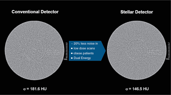
More recently, CT vendors have improved the design of their scintillation detectors for improved performance during imaging by using complex rare earth materials to function as activators in the scintillators used to capture and convert x-ray photos into light. For example, while GE uses a lutetium (Lu)-based garnet in their Gemstone CT detector array, Canon Medical Systems uses a praseodymium-activated scintillator in their PureViSION CT detector array. Furthermore, the more recent design considerations of CT detectors also include miniaturized detector electronics through the use of integrated DAS circuits. The purpose of such design elements is to reduce electronic noise and to reduce power consumption. The reduction in electronic noise results in low image noise with very small signals. Fig. 12.42 illustrates the noise comparison between the Siemens StellarInfinity CT detector and a conventional CT detector. A more comprehensive description of CT detectors is provided in Chapter 4.
Performance properties of detectors
It is beyond the scope of this text to discuss the physical performance properties of CT detectors; however, Dowsett, 2006 emphasized that detectors for MSCT scanners should have several properties. These include a large dynamic range, high quantum absorption efficiency, high luminescence efficiency, good geometric efficiency, small afterglow, and high precision machinability. In addition, they noted that all detector elements must have a uniform response. Readers interested in these properties should refer to the work of Dowsett, 2006. Several of these properties are described further in Chapter 4.
Detector configuration
The term detector configuration “describes the number of data collection channels and the effective section thickness determined by the data acquisition system settings” (Dalrymple et al., 2007). MSCT detectors can be configured in several ways by combining various detector elements electronically (or binning) to produce the desired slice thickness required for the examination at the isocenter. In general, typical slice thicknesses that can be obtained include:
- • 2 × 0.5 mm, 4 × 1.0 mm, 4 × 5.0 mm, 2 × 8.0 mm, and 2 × 10 mm for four-slice adaptive array detector
- • 16 × 0.5 mm, 16 × 1.0 mm, and 16 × 2.0 mm for a 16-slice fixed array detector
- • 40 × 0.625 mm and 32 × 1.25 mm for a 40-slice fixed array detector
- • 64 × 0.5 mm and 32 × 1.0 mm for a 64-slice fixed array detector
The reader should consult the manufacturer data sheets for specific slice thicknesses offered by their scanners.
Slice thickness selection
As mentioned earlier, individual slice widths (Fig. 12.43) are generally defined by the number of detector elements grouped (or binned) into each data channel (Dalrymple et al., 2007). The smallest slice width available is determined by the smallest single detector element. An exception to this generalization occurs in the nonuniform array shown in Fig. 12.43, in which two 0.5-mm slices can be acquired by moving the collimator leaves inward so that only the inner half of the two central 1-mm elements are exposed to the x-ray beam. Similarly, four 1-mm slices are acquired by irradiating the two central elements and two-thirds of the adjacent 1.5-mm elements. Slice width is defined at the center of rotation (center of the gantry aperture), so the actual detector dimensions for that slice will be greater because of the magnification produced by beam divergence. The x-ray beam width, as defined by the prepatient collimators, will be approximately four times the slice width.
The slice, as defined by the tissue irradiated during the rotation of a multislice detector, is significantly different from that of a single-detector scanner (Fig. 12.44). This is an extension of the problem with the earlier dual-detector scanners. In this case, however, the outer two slices are considerably more affected by beam divergence than are the inner two slices.
The significance of this geometric nonuniformity may be most severe in the case of conventional scanning. Reconstruction of the CT image involves all views acquired throughout the 360 degrees of data collection. When views from different angles are actually measuring quite different tissue pathways, there will be varying degrees of volume averaging with an increased likelihood of artifact and inaccurate reconstruction. If detector size is increased in future scanners to add more slices, this geometric situation will be further exaggerated. With the x-ray beam fan extended in the z-axis, as well as the x-y plane, a reconstruction algorithm different than those used for single-slice scanners is needed to process the raw data (Hu, 1999; Taguchi & Aradate, 1998).
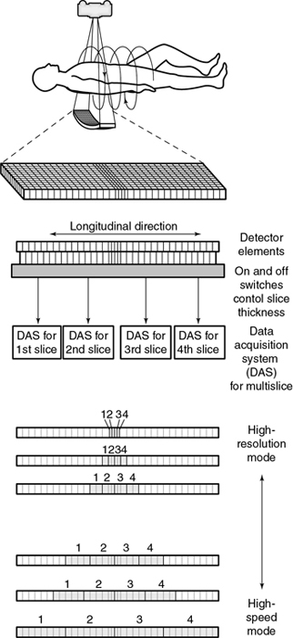
The signals from the individual detector elements are fed to four DASs through a bank of switches that combines the signals from the appropriate number of elements into the slice width selected by the operator (Fig. 12.45).
Detector elements outside the selected slices are switched off and do not contribute any signal to the DAS. Patient dose is controlled by prepatient collimators that restrict the x-ray beam to only those detector elements needed for the four data slices. At present, the slice thickness must be selected before scanning, and it is not possible to narrow the slice width after data collection. Summing slices after scanning to create fewer thicker images is certainly feasible and can have clinical value. In this case, it would be possible to return to the thinner slices if clinically indicated and if the raw data were still available.
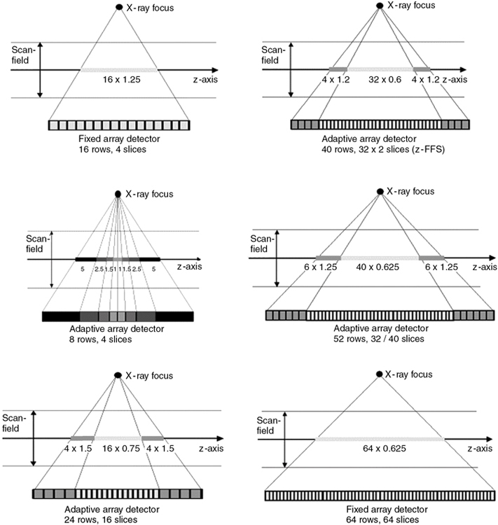
Fig. 12.46 provides examples of various combinations of detector elements for both fixed array and adaptive array detectors for MSCT imaging.
The design of the multirow detector influences the speed of acquisition of the slices and the resolution of the slices, as shown in Fig. 12.47.
Data acquisition system
Another major component of the gantry is the DAS, the detector electronics responsible mainly for digitizing the signals from the detectors before they are sent to the computer for processing. Figure 12.47 shows an example of a DAS coupled to the multirow detector array by switches. In this case, four slices are acquired at the same time because of the presence of four DAS systems (four times the electrical circuits compared with SSCT systems; Saito, 1998). Regardless of which four slices are required for the examination, the switches can be turned on and off to ensure that the appropriate detector segments are exposed to x rays.
Patient table
The patient table, or couch, features are essentially similar to those associated with SSCT and conventional step-and-shoot CT scanners. The purpose of the table is to support the patient and to facilitate MSCT scanning through the variable speed of travel of the tabletop and its wide range of movement. The table can be raised and lowered to accommodate positioning of the patient in the gantry aperture and to facilitate easy transfer of the patient from the scanner to a bed or gurney and vice versa. Movement of the tabletop in the longitudinal direction also facilitates patient position in the gantry aperture, with variable scannable ranges.
Patient tables for CT are equipped with a head holder or headrest to ensure patient comfort during the examination. In an emergency during the examination, the movement of the table can be controlled manually to ensure patient safety.
Computer system
The computer system for MSCT receives data from the DAS and the operator, who inputs patient data and various examination protocols. These systems must be capable of handling vast amounts of data collected by the 2D multirow detector array. These computers have hardware architectures that provide high-speed preprocessing, image reconstruction, and postprocessing operations. Although preprocessing includes various corrections to the raw data, image reconstruction refers to the use of multislice reconstruction algorithms for image buildup. On the other hand, postprocessing involves the use of a wide range of image processing and advanced visualization software, such as the generation of 3D and MPR, as well as virtual endoscopic images from the axial dataset stored in the computer.
All MSCT scanners now incorporate iterative reconstruction algorithms (see Chapter 6), which play a significant role in CT dose optimization. Furthermore, CT computer architectures also now include the graphics processing units (GPUs) for the simple reason that they can be used to reduce the processing requirements of the CPU. As reviewed by Pratx and Xing (2011), the GPU is now used in image reconstruction, image processing, dose calculation and treatment plan optimization, radiation treatment planning, and in other applications. Chapter 7 provides a further description of the role of the GPU in MSCT scanners. Furthermore, and as noted in Chapter 6, iterative reconstruction algorithms are now available on all MSCT scanners (Kalender, 2014). This marks what has been described as a “new era” in CT dose optimization, and recent studies have shown improved CT image quality at reduced dose compared with FBP algorithms (Kordolaimi et al., 2013). Buxi et al. (2014) showed that the average dose reduction for the thorax, abdomen/pelvis, and trunk examinations were estimated at 33.2%, 32.45%, and 49.70%, respectively.
The results of computer processing are displayed for viewing by an observer on a monitor. Several characteristics of the monitor are important to the observer, such as the display matrix, bandwidth, display memory, and the gray level and color resolution.
Data storage devices for holding the raw data and image data include hard disks, usually of the Winchester type with high storage capacities, and erasable optical disks of the magneto-optical type.
Operator console
The operator console allows the operator to interact with the scanner before, during, and after the examination. Essentially the major components include the keyboard, mouse, monitor, and other controls for the execution of specialized functions.
The operator console controls the entire CT scanner system and facilitates the selection of scan parameters and scan control (automatic or manual), image storage, communication, image reconstruction, image processing, windowing, control of the gantry, and x-ray tube rotation. The console allows for communication of images to other parts of the department and hospital and other remote sites through the use of local and wide-area networks. The MSCT console also supports full digital imaging and communication in medicine (DICOM) connectivity to other equipment, such as network printers. MSCT consoles also provide for the use of a wide range of software options for image processing, such as 3D imaging, virtual endoscopy, MIP, MPR reconstruction, cardiac applications, and dental CT and bone mineral analysis.
Isotropic imaging
One of the major goals of developing scanners with an increasing number of slices (4, 8, 16, 32, 40, 64, 320, and 640 slices) per rotation of the x-ray tube and detectors around the patient is to achieve isotropic imaging.
Definition
Several technical developments in MSCT scanners have made it possible to perform isotropic imaging. The term isotropic is used to refer to the size of the voxels used in a volume dataset. When the slice thickness is equal to the pixel size, all dimensions of the voxel (x, y, z) are equal. In other words, the voxel is a perfect cube, and the dataset acquired is said to be isotropic. If, however, all voxel dimensions are not equal, that is, the slice thickness is not equal to the pixel size, the dataset acquired is said to be anisotropic. The geometry of both isotropic and anisotropic data is clearly illustrated in Fig. 1.17.
Goals
One of the major goals of isotropic imaging in CT is to achieve excellent spatial resolution (detail) in all imaging planes, especially in MPR and 3D imaging. There are other benefits as well (Dalrymple et al., 2007; Paulson et al., 2004, 2005), but at the expense of more dose to the patient. Furthermore, the use of narrow collimation increases the scanning time. As noted by Dalrymple et al. (2007), “the parameters that affect the radiation dose and exposure time vary considerably according to scanner design and these variations determine the proportions of the trade-off in increased radiation dose and scanning time relative to the voxel size.” Therefore, in MSCT scanning, personnel should have a working knowledge of how voxel size affects not only the spatial resolution but also the radiation dose. Such understanding ensures that personnel work within the ALARA (as low as reasonably achievable) philosophy to optimize the image quality and radiation dose.
Data acquisition
Isotropic imaging with 4-, 16-, 40-, and 64-channel MSCT scanners has been described in some detail by Dalrymple et al. (2007). One of the major technical parameters that has an effect on isotropy is the detector configuration, that is, how the detector elements are used together with the effective slice thickness. Although the 4-channel MSCT scanner can achieve near isotropic imaging, the 16-, 32-, 40-, and 64-channel MSCT scanners can produce isotropic voxels, achieving isotropy. As demonstrated by Dalrymple et al. (2007), the scanners (beyond 4-slice) can also produce voxels that are anisotropic.
Image quality considerations
Image quality in CT is described in detail in Chapter 9. Essentially there are three main parameters: spatial resolution, contrast resolution, and noise. Spatial resolution, the ability of the scanner to image fine detail, is measured in line pairs per centimeter. Contrast resolution (or low-contrast resolution) or tissue resolution is the ability of the scanner to discriminate small differences in tissue contrast. Noise, on the other hand, is a fluctuation of CT numbers from point to point in the image for a scan of uniform material such as water. Noise degrades image quality and affects the perceptibility of detail. Artifacts can also degrade image quality and cause problems in image interpretation.
In MSCT, these parameters are the same in terms of definition. The purpose of MSCT is to improve on the performance of SSCT in terms of speed and coverage. The volume coverage speed performance in MSCT is better than its counterpart in SSCT without compromising image quality.
In addition, image quality depends on radiation dose. Although the dose in CT has received increasing attention in the literature and has been identified as an increasing source of radiation exposure and may be viewed as “a public health issue in the future” (Brenner & Hall, 2007), there have been increasing technical efforts to reduce this dose not only to adults but to children in particular. One such dose reduction technology is the tube current modulation techniques introduced by manufacturers. Dose in CT is described in detail in Chapter 10.
Acceptance testing and research studies will provide verification on image quality parameters and more information on the performance of MSCT scanners in the image quality and radiation dose arenas.
Wide area detector CT
Limitations of previous MSCT scanners
The technical evolution of MSCT scanners from 16-slice, 32-slice, 40-slice, and 64-slice CT scanners has resulted in numerous clinical benefits not only for enhancing diagnosis but also for use in radiation therapy and surgical simulation. One such benefit of MSCT imaging is improved three-dimensional (3D) CT (3D CT) imaging of anatomic structures; however, a notable problem was to obtain dynamic 3D CT images of the beating heart in cardiac imaging. In addition, these MSCT scanners can increase the dose to patients (Brenner & Hall, 2007), create image artifacts especially in cardiac CT imaging as a result of the beating heart, and have limited organ coverage because of the size of the detector (20 mm to 40 mm). The latter implies that two or more rotations are needed to cover the entire organ, such as the heart or lungs.
What is wide area detector CT? Four-dimensional CT imaging
To solve these problems, other CT scanners referred to as area detector CT (ADCT), also referred to as wide area detector CT (WADCT), were developed to obtain dynamic 3D CT of the beating heart (Katada & Clouse, 2015). Dynamic 3D CT is referred to as 4D CT imaging (Mori et al., 2004, personal communications). Later, other workers such as Kwong et al. (2015) and Buzzatti et al. (2019) described and used 4D imaging in other clinical applications. Kwong et al. (2015) for example, provided a more detailed definition of 4D CT imaging as “a three-dimensional computed tomography volume containing a moving structure is imaged over a period of time, creating a dynamic volume data set. 4DCT has previously been mainly utilized in the setting of radiation therapy planning, but with the development of wide field of view CT, 4DCT has opened major avenues in the diagnostic arena.”
Development of wide area detector CT
The history of the development of WADCT is marked by the development of two special MSCT scanners; the 256-slice and 320-slice CT scanners, and described in detail by Katada and Clouse (2015). The 256-slice scanner is described in the next subsection and lays the foundations for the 320-slice scanner.
The 256-slice beta four-dimensional CT scanner
The first model of the 256-slice 4D CT scanner was developed at the National Institute of Radiological Sciences in Japan in 2003 (Mori et al, 2004: personal communications). The major goal of this scanner is to produce 4D CT images with a wide-area detector capable of covering the entire organ (heart or lung) in a single rotation rather than multiple rotations.
The second model of the 256-slice 4D CT scanner (Fig. 12.48A) is based on the design of the first model, and in 2006 and 2007 this model prototype scanner was installed in three centers for clinical beta trials (Fujita Health University, Nagoya, Japan; National Cancer Center, Tokyo, Japan; and Johns Hopkins University, Baltimore, Maryland).
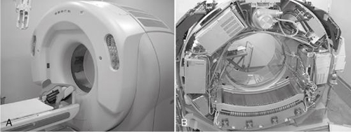
The most conspicuous difference is the use of a wide-area 2D detector mounted on the gantry frame of a 16-slice CT scanner (Canon Medical Systems, formerly Toshiba Medical Systems, Japan), as shown in Fig. 12.48B. The scanner uses a cone beam with a larger cone angle (about 13 degrees) compared with the previous MSCT scanners to cover a wider FOV. The total beam width is 128 mm, four times the size of the Aquilion 16-slice CT scanner (Canon Medical Systems, formerly Toshiba Medical Systems-Japan). This wide beam ensures complete coverage of the entire organ (heart) in one complete rotation (Fig. 12.49).
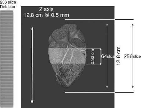
The 256-slice 4D CT scanner has 912 (transverse) × 256 (craniocaudal) detector elements, each approximately 0.5 mm × 0.5 mm at the center of rotation. The 128-mm total BW allows for the continuous use of several collimation sets. The detector element is made of a gadolinium oxysulfide and a single crystal silicon photodiode as used in the current MSCT scanners.
The rotation time is 0.5 seconds per rotation and the dynamic range is 18 bits. The reconstruction algorithm used in this scanner is the Feldkamp cone-beam algorithm. Real-time reconstruction processing is done by 32-field programmable gate arrays (FPGSs-Virtex II Pro, Xilinx, San Jose, CA) with a clock speed of 125 MHz. volumes of 256 × 256 × 128 can be produced.
The clinical beta testing program of the 256-slice CT scanner laid the foundations for the design of a new MSCT scanner designed to image the entire heart in a single rotation. This scanner is Canon’s 320-slice Aquilion ONE Dynamic Volume CT scanner (Canon Medical Systems, formerly Toshiba Medical Systems-Japan), which is described briefly in the next section.
The 320-slice dynamic volume CT scanner
In 2007, the 320-slice 4D CT scanner, referred to as the Aquilion ONE MSCT scanner was introduced at the RSNA meeting in Chicago. The gantry, patient table, and display workstations of the 320-slice dynamic volume CT scanner are illustrated in (Fig. 12.50). One of the characteristic technical features of this scanner is its wide-area 2D detector, which ensures a field coverage of 160 mm (compared with 128 mm of the 256-slice prototype CT scanner). The detector is designed with a number of detector rows with 320 ultrahigh resolution detector elements. This feature allows for scanning the entire anatomical structures such as the heart, lungs, and brain in a single rotation; therefore, it does not require the spiral/helical scanning principle.
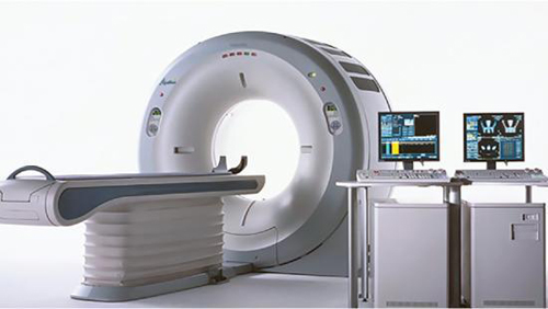
This high-speed volume scanner features a rotation time of 350 ms, which is needed to provide a temporal resolution for imaging the entire heart in one heartbeat with excellent spatial and contrast resolution at lower doses (Mather, 2007). In addition, the reconstruction time is fast (less than 10 seconds) and is made possible through the use of specially designed reconstruction processors.
A major challenge in the development of this wide-area detector CT volume scanner is the large cone angle because the beam divergence is much greater than that of the 256-slice scanner. While it is 3 degrees for a 64-slice scanner, it is 15 degrees for the 320-slice scanner. To address this problem (greater beam divergence for the 320-slice scanner) Toshiba developed an FDK-based algorithm called the coneXact reconstruction algorithm, which eliminates any cone-beam image artifacts.
The 320-slice volume scanner can be used in neurological imaging, including whole-brain CT perfusion studies, to reduce “the chances of misregistration of lesions regardless of location, and makes the selection of the arterial input function easy” (Shankar & Lum, 2011), and in perfusion studies (Motosugi et al., 2012), CT angiography (Gang et al., 2012; Luo et al., 2012; Qin et al., 2012; Tatsugami et al., 2012; Tomizawa et al., 2012), cardiopulmonary imaging (Yang et al., 2012), and other applications, such as in pediatric imaging (Sorantin et al., 2013), where entire organs (chest, for example) can be scanned very quickly. Such scanning results in large datasets that will provide more information for the radiologist to use in diagnostic management of the patient.
More recently, Kang (2019) provided an update of the clinical applications of WADCT scanners for cardiothoracic imaging and offered the following conclusion:
Wide-detector CT scanners provide advantages in terms of improvement in image quality and reduction of the radiation dose and contrast material volume in routine CCTA examination than in conventional 64- or 128-detector row scanners. Moreover, given their unique characteristic of z-axis coverage, several new technologies [such as myocardial function/perfusion, Transluminal attenuation gradient (TAG) or subtraction imaging] have become more feasible and better reflect the exact physiological status of patients. Further development of wide-detector CT scanners, especially for improvements in temporal and spatial resolutions (with faster rotation times and thinner individual detector widths), may provide great clinical advantages in the future.
Double-slice technology: 640 slices per rotation
Double-Slice Technology is a major feature of the 320-slice 4D CT scanner (Canon’s Aquilion ONE CT scanner) in which 640 slices per rotation can be obtained. For example, with 0.5 mm slice thickness and 0.25 mm interval, the 320-slice scanner detector rows will generate 640 slices per rotation, as illustrated in Fig. 4.44.
The double-slice technology utilizes a special 3D image reconstruction algorithm referred to as the coneXact 3D volume reconstruction algorithm, which takes into account the wider beam divergence (15 degrees) of the 320-slice 4D scanner. It is not within the scope of this book to describe the details of the coneXact image reconstruction; however, the interested reader may refer to Blobel et al. (2009) for more technical information.
Dual-source CT: Basic principles
Evolution at a glance
In 2006, a CT scanner primarily designed for cardiac imaging (and other applications as well) was introduced at the RSNA meeting. This scanner, referred to as the dual-source CT (DSCT) scanner introduced by Siemens Medical Solutions, now referred to as Siemens Healthineers (Forchheim, Germany), featured a unique design incorporating two x-ray tubes coupled to two detector systems that provided a scanner with two DASs.
CT imaging of the heart with MSCT scanners dates back to 1999, and because the heart is in constant motion (beating heart), temporal resolution is essential to avoid motion artifacts. Additionally, for cardiac imaging with CT, it is important to cover the entire heart in a single breath-hold. Although four-slice CT scanners provided acceptable results, problems with respect to motion artifacts, greater heart rates, long breath-hold times, and limited spatial resolution still persisted (Flohr et al., 2006).
The introduction of 16-slice scanners provided improved gains in spatial and temporal resolution compared with four-slice systems. The subsequent arrival and use of 64-slice CT scanners provided further improvements in the technical requirements for cardiac imaging. For example, these scanners provided spatial resolution (by isotropic imaging) and temporal resolution because of the reduction of gantry rotation times to 0.33 ms (necessary to deal with high rates) compared with about 0.375 seconds for 16-slice scanners (Flohr et al., 2006). One of the problems in CT cardiac imaging is removing the need for heart rate control; therefore, efforts are needed to improve temporal resolution below 100 ms at any heart rate, such as 66 ms for example (Parakh et al., 2021).
Major technical components
The major system components of the DSCT scanner are illustrated in Fig. 12.51. The most noticeable difference between this scanner and other MSCT scanners is that there are two DASs offset by 90 degrees (Engel et al., 2008). While the acquisition system labeled “Det A” has a large scan FOV diameter, the acquisition system labeled “Det B” has a smaller scan FOV diameter.
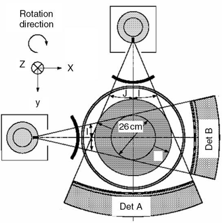
Modes of operation
A major advantage of two acquisition systems, is that DSCT can operate in two modes, namely a dual-source single-energy (DSSE) mode, and a dual-source dual-energy (DSDE) mode. Whereas in the DSSE mode both x-ray tubes are energized using the same kV setting, and provide “extremely fast volumetric coverage providing both the power and speed for imaging very obese patients, whole body trauma and cardiac imaging” (Parakh et al., 2021), in the DSDE mode, the x-ray tubes operate “at different energies to provide the maximum spectral separation, which is the key to high sensitivity and specificity in spectral imaging” (Parakh et al., 2021).
Another term used to describe DSCT is dual-energy CT (DECT) defined as “the use of attenuation measurements acquired with different energy spectra, along with use of the known changes in attenuation between the two spectra, to differentiate and quantify material composition.”
Cardiac CT imaging
One important reason for using the DSCT scanner operating in the DSSE mode is related to the cardiac imaging requirements where the optimum temporal resolution is mandatory. Such resolution is needed to reduce motion artifacts created by the beating heart. Although it is not within the scope of this chapter to describe the details of cardiac CT imaging, the interested reader may refer to Forghani et al. (2017).
Spectral CT imaging
The DSDE operational mode of the DSCT scanner can provide CT data with two different energy spectra. This is sometimes referred to as spectral CT imaging or multienergy CT imaging (only two different energy spectra). Multienergy CT imaging can be accomplished using photon-counting detector CT and multienergy CT postprocessing (Rajiah et al., 2020). For a detailed description of photon counting CT, the interested reader may refer to an article by Willemink et al. (2018).
Other imaging applications
Other applications of the DSCT scanner include the following: DSCT has been used in abdominopelvic imaging (Coursey et al., 2010), CTA of the supra-aortic arteries (Lell et al., 2010), abdominal imaging (Silva et al., 2011), imaging in the genitourinary tract (Kaza et al., 2012), pulmonary hypertension (Ameli-Renani et al., 2014), CT of the abdomen (Marin et al., 2014), CT colonography (Karcaaltincaba & Ozdeniz, 2014), and in children (Siegel & Ramirez-Giraldo, 2019).
Advantages of MSCT
MSCT offers a wide range of both technical and clinical advantages. Since the introduction of MSCT a number of advantages have been outlined by Saito (1998), as well as by Kohl (2005), Kalender (2005), Mather (2005b), Douglas-Akinwande (2006), Kachelriess et al., 2006, and Cody and Mahesh (2007). There are several technical factors in MSCT scanning that combine to improve not only the spatial and contrast resolution of images but also the temporal resolution (fewer motion artifacts). Furthermore, MSCT opens up improved gains in other clinical applications, including CT imaging in emergency and ICU settings, CT imaging in trauma, abdominal and pelvic imaging, pulmonary imaging, cardiovascular imaging, musculoskeletal imaging, neurological and head and neck imaging, and CT-guided interventional procedures (Ghonge, 2013). Furthermore, MSCT offers improved MPR images and 3D-rendered images, retrospective creation of thinner or thicker sections from the same raw data, and delivery of intravenously administered iodinated contrast material at faster rates, and so on.
Specifically, these advantages include the following:
- 1. Increase in speed and volume coverage. In MSCT, the increase in pitch and the increase in rotation speed of the x-ray tube and detectors allow for a larger volume of the patient to be scanned in less time. Hu (1999), for example, showed that a four-slice helical/spiral CT scanner is about two times faster than an SSCT scanner for comparable image quality.
- 2. Improved spatial resolution. MSCT images thin slices with better isotropic resolution. This is sometimes referred to as isotropic imaging (described earlier in the chapter), in which case all the sides (axial, vertical, and horizontal) of the voxels in the slice have equal dimensions compared with SSCT. This advantage provides improved MPR and 3D images with reduced image artifacts.
- 3. Efficient use of the x-ray beam. In MSCT, the x-ray beam width has to be opened to fall on the 2D detector array compared with a single-row detector array characteristic of SSCT scanners. The entire beam is thus used to acquire four slices (images) per 360-degree rotation without wasting any portion of the x-ray beam, as opposed to one slice per 360-degree rotation in the SSCT case, in which a portion of the x-ray beam is wasted during data acquisition. Such use of the beam increases the life of the x-ray tube. The tube can now be used to produce a large number of thin slices without having to wait for it (x-ray tube) to cool, a problem with SSCT systems. In 1999, Kopecky et al. (1999) noted that with an x-ray tube with a lifespan of 200,000 seconds, a SSCT scanner will provide about 200,000 images (one image per second) compared with 800,000 images for a four-slice MSCT scanner (same conditions are maintained), “or 1.6 million images if the gantry spins at two revolutions per second, or 3.2 million images if two images are created for each full rotation of 0.5 secs.”
- 4. Reduction of radiation exposure. The development of new dose reduction technology such as tube current modulation techniques (Kanematsu et al., 2015; McNitt-Gray, 2011) and the recent use of iterative reconstruction algorithms (Buxi et al., 2014; Kalender, 2014; Kordolaimi et al., 2013; Chapter 6) will play a significant role in CT dose reduction.
- 5. Improved accuracy in needle placement in CT fluoroscopy. One of the problems with needle placement under CT fluoroscopic control with an SSCT scanner is illustrated in Fig. 12.52. The image shows that the needle has hit the target, which is simply not the case. This problem is solved with MSCT scanners that offer CT fluoroscopy because multiple images are obtained. It is apparent in Figure 12.52 that the target has been hit.
- 6. Cardiac CT imaging. MSCT technology has been developed to such a level that “dedicated” CT scanners for imaging the heart such as the DSCT scanner and the 320-slice 4D CT scanner. These scanners can image the heart (and other organ systems) with exceptional spatial, contrast, and temporal resolution, as well as with reduced doses compared with 64-slice CT scanners. Additionally, the use of special cardiac reconstruction algorithms can have an impact on artifact reduction when the beating heart is imaged (Cody & Mahesh, 2007; Dowe, 2006; Flohr, 2006; Flohr et al., 2006; Kachelriess et al., 2006; Mather, 2005b, 2007; Primak et al., 2006).
- 7. Spectral CT Imaging (Rajiah et al., 2020; Willemink et al., 2018).
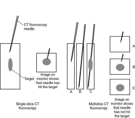
Review questions
Answer the following questions to check your understanding of the materials studied.
- 1. The limitations of conventional CT are:
- 2. The shortcomings of single-slice volume CT imaging are:
- 3. The definition of pitch in a multislice scanner, as defined by the International Electrotechnical Commission, states:
- 4. Pitch directly relates to:
- 5. In multislice computed tomography, a ________________ beam geometry results, rather than a fan beam as in single-slice computed tomography scanners.
- 6. As the pitch increases, the image quality:
- 7. In a multislice computed tomography scanner, what type of algorithm can be used if the number of detector rows is small?
- 8. All of the following are materials used in solid-state detectors except:
- 9. What term is used to describe the number of data collection channels and the effective section thickness determined by the data acquisition system settings?
- 10. When the slice thickness is equal to the pixel size, the data acquired are said to be:
References
Ameli-Renani S, Rahman F, Nair A., et al. Dual-energy CT for imaging of pulmonary hypertension: Challenges and opportunities Radiographics 2014;34: 1769-1790.
Baker C.C.T. Dictionary of mathematics 1961; Hart New York.
Blobel J, Mews J, DeVries H, Irwan R. & Ogawa Y. Double slice mode for CT image reconstruction Visions Magazine 9, 2009;14: Japan, Toshiba Medical Systems.
Brenner D.J. & Hall E.J. Computed tomography—an increasing source of radiation exposure New England Journal of Medicine 2007;357: 22.
Bresler Y. & Skrabacz C. Optimal interpolation in helical scan 3D computerized tomography 1993; National Science Foundation MIP88-10412 1472-1475.
Bushong S. Radiologic science for technologists 11th ed. 2017; Philadelphia, PA Mosby.
Buxi T.B.S, Yadav A, Singh R.K. & Ghuman S.S. Effect of iterative reconstructions in low dose computed tomography Journal of Biomedical Graphics and Computing 3, 2014;4: 1-9.
Buzzatti L, Keelson B, Apperloo J., et al. Four-dimensional CT as a valid approach to detect and quantify kinematic changes after selective ankle ligament sectioning Scientific Reports 2019;9: 1291. https://doi.org/10.1038/s41598-018-38101-5.
Chen L, Liang Y. & Heuscher D.J. General surface reconstruction for cone-beam multislice spiral computed tomography Medical Physics 2003;30: 2804-2812.
Cody D.D. & Mahesh M. Technologic advances in multi-slice CT with a focus on cardiac imaging Radiographics 2007;27: 1829-1837.
Coursey C.A, Nelson R.C, Boll D.T., et al. Dual-energy multidetector CT: How does it work, what can it tell us, and when can we use it in abdominopelvic imaging? RadioGraphics 4, 2010;30: 1037-1055.
Dalrymple N.C, Prasad S.R, El-Merhi F.M. & Chintapalli K.N. Price of isotropy in multidetector CT Radiographics 2007;27: 49-62.
Douglas-Akinwande A.C, Buckwalter K.A, Rydberg J, Rankin J.L. & Choplin R.H. Multichannel CT: Evaluating the spine in postoperative patients with orthopedic hardware Radiographics 2006;26: S97-S110.
Dowe D.A. Prospectively gated CTA dramatically reduces dose Diagnostic Imaging 2006;28: S1-S5.
Dowsett D. The physics of diagnostic imaging 2006; Hodder Arnold London.
Engel K.J, Hermann C. & Zeitler G. X-ray scattering in single- and dual-source CT Medical Physics 2008;35: 318-332.
Feldkamp L.A, Davis L.C. & Kress J.W. Practical cone-beam algorithm Journal of the Optical Society of America 1984;1: 612-619.
Flohr, T.G. (2006). Radiation dose with dual source CT. June 94–97 Siemens Medical Solutions June 94–97.
Flohr T.G, Schaller S, Stierstorfer K., et al. Multi-detector row CT systems and image reconstruction techniques Radiology 2005;235: 756-773.
Flohr T.G, McCollough C.H, Bruder H., et al. First performance of a dual-source CT PSCT system European Journal of Radiology 2006;16: 256-268.
Forghani R, De Man B. & Gupta R. Dual-energy computed tomography physical principles, approaches to scanning, usage, and implementation: Part 1 Neuroimaging Clinics of North America 2017;27: 371-384.
Fukuda A, Lin P.J, Matsubara K. & Miyati T. Measurement of table feed speed in modern CT Journal of Applied Clinical Medical Physics 3, 2014;15: 275-281 https://doi.org/10.1120/jacmp.v15i3.4703.
Gang S, Min L, Li L., et al. Evaluation of CT coronary artery angiography with 320-row detector CT in a high-risk population British Journal of Radiology 2012;85: 562-570.
Ghonge N.P. Computed tomography in the 21st century: Current status and future prospects Journal of the International Medical Sciences Academy 1, 2013;26: 35-42.
He, H. D. (1999). Personal communication, General Electric Medical Systems.
Hsieh, J, Nett, B, Yu, Z.et al. (2013). Recent advances in CT image reconstruction Current Radiology Reports, Published online. doi: 10.1007/g40134-012-0003-7.
Hu H. Multislice helical CT: Scan and reconstruction Medical Physics 1999;26: 5.
IEC & (International Electrotechnical Commission). Medical Electrical Equipment-60601 Part 2-44: Particular requirements for the safety of x-ray equipment for computed tomography 1999; Geneva. IEC Switzerland.
James, G, & James, R. (Eds.). Mathematics dictionary (4th ed.). New York: Van Nostrand Reinhold.
Kachelriess M. Clinical x-ray computed tomography W. Schlegel, et al. New technologies in radiation oncology 2006; Springer New York.
Kalender W.A. Spiral CT scanning for fast and continuous volume data acquisition W.A. Fuchs. Advances in CT 1990; Springer-Verlag New York.
Kalender W.A. Spiral or helical CT: Right or wrong? Radiology 1994;193: 583.
Kalender W.A. Principles and performance of spiral CT L.W. Goldman & J.B. Fowlkes. Medical CT and ultrasound: Current technology and applications 1995; College Park, MD American Association of Physics in Medicine.
Kalender W.A. Computed tomography: Fundamentals, system technology, image quality, applications 2005; Erlangen, Germany Publicis Corporate Publishing.
Kalender W.A. Dose in x-ray computed tomography Physics in Medicine and Biology 2014;59: R129-R150.
Kanematsu M, Kondo H, Miyoshi T., et al. Whole-body CT with high heat-capacity X-ray tube and automated tube current modulation—effect of tube current limitation on contrast enhancement, image quality and radiation dose European Journal of Radiology 5, 2015;2084: 877-883 doi: 10.1016/j.ejrad.2015.01.019.
Kang E.J. Clinical applications of wide-detector CT scanners for cardiothoracic imaging: An update Korean Journal of Radiology 12, 2019;20: 1583-1596 https://doi.org/10.3348/kjr.2019.0327.
Karcaaltincaba M. & Ozdeniz I. Dual-energy CT for diagnostic CT colonography Radiographics 2014;334: 847-848.
Katada, K. Clouse & M.E. Area detector CT 2015; Medical Tribune Tokyo, Japan.
Kaza R.K, Platt J.F, Cohan R.H., et al. Dual-energy CT with single- and dual-source scanners: Current applications in evaluating the genitourinary tract Radiographics 2012;32: 353-369.
Kohl G. The evolution and state-of-the-art principles of multi-slice computed tomography Proceedings of the American Thoracic Society 2005;2: 470-476.
Kopecky K, Buckwalter K.A. & Sokiranski R. Multislice CT spirals pass single-slice in diagnostic efficacy Diagnostic Imaging 1999;21: 36-42.
Kordolaimi S.D, Argento S, Pantos I., et al. A new era in computed tomography dose optimization: The impact of iterative reconstruction on image quality and radiation dose Journal of Computer Assisted Tomography 6, 2013;37: 924-931.
Kudo, H, & Saito, T. (1991). Helical-scan computed tomography using cone-beam projections. In IEEE Conf. Record 1991 Nuclear Science Symposium and Medical Imaging Conference (pp. 1958–1962). Santa Fe, New Mexico.
Kwong Y, Mel A.O, Wheeler G. & Troupis J.M. Four-dimensional computed tomography (4DCT): A review of the current status and applications Journal of Medical Imaging and Radiation Oncology 5, 2015;59: 545-554 doi: 10.1111/1754-9485.12326.
Lell M.M, Hinkmann F, Nkenke E., et al. Dual energy CTA of the supraaortic arteries: Technical improvements with a novel dual source CT system European Journal of Radiology 2, 2010;76: e6-e12.
Liang Y. & Kruger R.A. Dual-slice spiral versus single-slice spiral scanning: Comparison of the physical performance of two computed tomography scanners Medical Physics 1996;23: 205-217.
Lu F, Gao Y, Kong Q, Qiao P, Shao M. & Xie M. Application of 640-slice CT wide-detector volume scan in low-dose CT pulmonary angiography Journal of X-ray Science and Technology 2, 2019;27: 197-205 doi: 10.3233/XST-180427.
Luo Z, Wang D, Sun X., et al. Comparison of the accuracy of subtraction CT angiography performed on 320-detector row volume CT with conventional CT angiography for diagnosis of intracranial aneurysms European Journal of Radiology 1, 2012;81: 118-122.
Marin D, Boll D.T, Mileto A. & Nelson R.C. State of the art: Dual-energy CT of the abdomen Radiology 2, 2014;271: 327-342.
Mather, R. (2005). Patient focused imaging—Aquilion’s low dose vision. July 4–8 Toshiba Med Rev 17.
Mather, R. (2005a). Meeting the cone-beam challenge—Aquilion’s sureCardio™ and TCOT. Toshiba Med Rev October 15, 16–21.
Mather R. Aquilion ONE—dynamic volume computed tomography 2007; Toshiba Medical Systems.
McNitt-Gray, M. (2011). Tube current modulation approaches: Overview, practical issues and potential pitfalls AAPM 2011 Summit on CT dose. American Association of Physicists in Medicine.
Mori I. (1987). Computerized tomographic apparatus utilizing a radiation source U.S. Patent No. 4630202.
Mori S, Endo M, Tsunoo T., et al. Physical performance evaluation of a 256-slice CT-scanner for four-dimensional imaging Medical Physics 2004;31: 1348-1356.
Mori S, Endo M, Komatsu S, Kandatsu S, Yashiro T. & Baba M. A combination-weighted Feldkamp-based reconstruction algorithm for cone-beam CT Physics in Medicine and Biology 2006;51: 3953-3965.
Motosugi U, Ichikawa T. & Sou H. Multi-organ perfusion CT in the abdomen using a 320-detector row CT scanner: Preliminary results of perfusion changes in the liver, spleen, and pancreas of cirrhotic patients European Journal of Radiology 10, 2012;81: 2533-2537.
Napel S.A. Basic principles of spiral CT E.D. Fishman, R.B. Jeffrey & Jr. Spiral CT: Principles, techniques, and clinical applications 1995; Raven Press New York.
Oxford English Dictionary. (2008). http://oed.com. Accessed September 19, 2008.
Ozaki M. Development of a real-time reconstruction system for CT fluorography Toshiba Medical Review 1995;53: 12-17.
Parakh A, Lennartz S, An C., et al. Dual-energy CT images: Pearls and pitfalls Radiographics 1, 2021;41: 98-119.
Paulson E.K, Jaffe T.A, Thomas J, Harris J.P. & Nelson R.C. MDCT of patients with acute abdominal pain: A new perspective using coronal reformations from submillimeter isotropic voxels American Journal of Roentgenology 2004;183: 899-906.
Paulson E.K, Harris J.P, Jaffe T.A, Haugan P.A. & Nelson R.C. Acute appendicitis: Added diagnostic value of coronal reformations from isotropic voxels at multi-detector row CT Radiology 2005;235: 879-885.
Pratx G. & Xing L. GPU computing in medical physics: A review Medical Physics 5, 2011;38: 2685-2687.
Primak A.N, McCollough C.H, Bruesewitz M.R, Zhang J. & Fletcher J.G. Relationship between noise, dose, and pitch in cardiac multi-detector row CT Radiographics 2006;26: 1785-1794.
Qin J, Liu L.Y, Fang Y., et al. 320-detector CT coronary angiography with prospective and retrospective electrocardiogram gating in a single heartbeat: Comparison of image quality and radiation dose British Journal of Radiology 2012;85: 945-951.
Rajiah P, Parakh A, Kay F, Baruah D. & Kambadakone A.R. Update on multienergy CT: Physics and applications Radiographics 5, 2020;40: 1284-1308.
Saito Y. Multislice x-ray CT scanner Medical Review 1998;66: 1-8.
Shankar J.J. & Lum C. Whole brain CT perfusion on a 320-slice CT scanner Indian Journal of Radiologic Imaging 3, 2011;21: 209-214.
Siegel M.J. & Ramirez-Giraldo J.C. Dual-energy CT in children: Imaging algorithms and clinical applications Radiology 2019;291: 286-297 https://doi.org/10.1148/radiol.2019182289.
Silva A.C, Morse B.G, Hara A.K., et al. Dual-energy (spectral) CT: Applications in abdominal imaging Radiographics 2011;31: 1031-1046.
Silverman P.M, Corboy K. & Zeman R.K. Helical vs spiral American Journal of Roentgenology 1994;162: 1247.
Sorantin E, Riccabona M, Stucklschweiger G, Guss H. & Fotter R. Experience with volumetric (320 rows) pediatric CT European Journal of Radiology 7, 2013;82: 1091-1097.
Taguchi K. & Aradate H. Algorithm for image reconstruction in multislice helical CT Medical Physics 1998;25: 550.
Tatsugami F, Matsuki M, Nakai G., et al. The effect of adaptive iterative dose reduction on image quality in 320-detector row CT coronary angiography British Journal of Radiology 2012;85: e378-e382.
Tohki Y. The helical scanning technique Toshiba Med Rev 1991;38: 1-5.
Tomizawa N, Komatsu S, Akahan M., et al. Influence of hemodynamic parameters on coronary artery attenuation with 320-detector coronary CT angiography European Journal of Radiology 2, 2012;81: 230-233.
Toshiba Medical Systems. (2008). Personal communications.
Towers M.J. Spiral geometries: The helix is one type of spiral. From spiral or helical CT? American Journal of Roentgenology 1993;161: 901.
Willemink M.J, Persson M, Pourmorteza A, Pelc N.J. & Fleischmann D. Photon-counting CT: Technical principles and clinical prospects Radiology 2018;289: 293-312 https://doi.org/10.1148/radiol.2018172656.
Yang L, Xu L, Yan Z., et al. Low dose 320-row CT for left atrium and pulmonary veins imaging—the feasibility study European Journal of Radiology 7, 2012;81: 1549-1554.