Dissolution and solubility
Michael E. Aulton
Chapter contents
Solution, solubility and dissolution
Energy/work changes during dissolution
Dissolution rates of solids in liquids
Factors affecting the rate of dissolution
Measurement of dissolution rates of drugs from dosage forms
Methods of expressing solubility and concentration
Solubility of solids in liquids
Solubility of gases in liquids
Solubility of liquids in liquids
Distribution of solutes between immiscible liquids
Key points
• Dissolution rate and solubility are two separate properties. While a chemical with a fast dissolution rate often has a high solubility (and vice versa), this is not always the case. The differences are explained in the chapter.
• The process of dissolution involves a molecule, ion or atom of a solid entering a liquid phase in which the solid is immersed.
• The rate of dissolution is controlled either by the speed of removal of the molecule, ion or atom from the solid surface or by the rate of diffusion of that moiety through a boundary layer that surrounds the solid.
• Various factors influence the rate of diffusion of a solute through boundary layers. Some of these may be manipulated by the formulator.
• It is important for the formulator to be aware of the parameters which affect the solubility of a solid in a liquid phase.
• The dissolution rate and solubility of solids in liquids, gases in liquids and liquids in liquids are each important to pharmaceutical science and these are discussed.
Introduction
Solutions are encountered frequently in pharmaceutical development, either as a dosage form in their own right or as a clinical trials material. Additionally, almost all drugs function in solution in the body.
This chapter discusses the principles underlying the formation of solutions from solute and solvent and the factors that affect the rate and extent of the dissolution process. This process will be discussed particularly in the context of a solid dissolving in a liquid as this is the situation most likely to be encountered in the formation of a drug solution, either during manufacturing or during drug delivery.
Further properties of solutions are discussed in Chapter 3 and 24. Because of the number of principles and properties that need to be considered, the contents of each of these chapters should only be regarded as introductions to the various topics. The student is encouraged, therefore, to refer to the bibliography cited at the end of each chapter in order to augment the present contents. The textbook written by Florence & Attwood (2011) is recommended particularly. It uses a large number of pharmaceutical examples to aid in the understanding of physicochemical principles.
Definition of terms
This chapter will begin by clarifying some of the key terms relevant to solutions.
Solution, solubility and dissolution
A solution may be defined as a mixture of two or more components that form a single phase that is homogeneous down to the molecular level. The component that determines the phase of the solution is termed the solvent; it usually (but not necessarily) constitutes the largest proportion of the system. The other component(s) are termed solute(s) and these are dispersed as molecules or ions throughout the solvent, i.e. they are said to be dissolved in the solvent.
The transfer of molecules or ions from a solid state into solution is known as dissolution. Fundamentally, this process is controlled by the relative affinity between the molecules of the solid substance and those of the solvent. The extent to which the dissolution proceeds under a given set of experimental conditions is referred to as the solubility of the solute in the solvent. The solubility of a substance is the amount of it that passes into solution when equilibrium is established between the solute in solution and the excess (undissolved) substance. The solution that is obtained under these conditions is said to be saturated. A solution with a concentration less than that at equilibrium is said to be subsaturated. Solutions with a concentration greater than equilibrium can be obtained in certain conditions; these are known as supersaturated solutions.
Since the above definitions are general ones, they may be applied to all types of solution involving any of the three states of matter (gas, liquid, solid) dissolved in any of the three states of matter, i.e. solid-in-liquid, liquid-in-solid, liquid-in-liquid, solid-in-vapour, etc. However, when the two components forming a solution are either both gases or both liquids, then it is more usual to talk in terms of miscibility rather than solubility. Other than the name, all principles are the same.
One point to emphasize at this stage is that the rate of solution (dissolution rate) and amount which can be dissolved (solubility) are not the same and are not necessarily related. In practice, high drug solubility is usually associated with a high dissolution rate, but there are exceptions; an example is the commonly used film-coating material hydroxypropyl methylcellulose (HPMC) which is very water soluble yet takes many hours to hydrate and dissolve.
Process of dissolution
Dissolution mechanisms
The majority of drugs and excipients are crystalline solids. Liquid, semi-solid and amorphous solid drugs and excipients do exist but these are in the minority. For now, we will restrict our discussion to dissolution of crystalline solids into liquid solvents. Also, to simplify the discussion, it will be assumed that the drug is molecular in nature. The same discussion applies to ionic drugs. Again, to avoid undue repetition in the explanations that follow, it can be assumed that most solid crystalline materials, whether drugs or excipients, will dissolve in a similar manner.
The dissolution of a solid in a liquid may be regarded as being composed of two consecutive stages.
1. First is an interfacial reaction that results in the liberation of solute molecules from the solid phase to the liquid phase. This involves a phase change so that molecules of solid become molecules of solute in the solvent in which the crystal is dissolving.
2. After this, the solute molecules must migrate through the boundary layers surrounding the crystal to the bulk of solution.
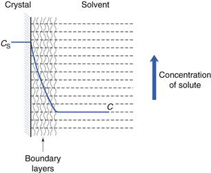
These stages, and the associated solution concentration changes, are illustrated in Figure 2.1.
These two stages of dissolution are now discussed in turn.
Interfacial reaction
Leaving the surface.
Dissolution involves the replacement of crystal molecules by solvent molecules. This is illustrated in Figure 2.2.
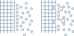
Fig. 2.2 Schematic representation of the replacement of crystal molecules with solvent molecules during dissolution.
The process of the removal of drug molecules from a solid, and their replacement by solvent molecules, is determined by the relative affinity of the various molecules involved. The solvent/solute forces of attraction must overcome the cohesive forces of attraction between the molecules of the solid.
Moving into the liquid.
On leaving the solid surface, the drug molecule must become incorporated in the liquid phase, i.e. within the solvent. Liquids are thought to contain a small amount of so-called ‘free volume’. This can be considered to be in the form of ‘holes’ that, at a given instant, are not occupied by the solvent molecules themselves (this point is discussed further in Chapter 3). Individual solute molecules are thought to occupy these ‘holes’, as shown in Figure 2.3.
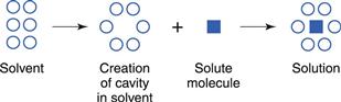
The process of dissolution may be considered, therefore, to involve the relocation of solute molecules from an environment where they are surrounded by other identical molecules, with which they form intermolecular attractions, into a cavity in a liquid where they are surrounded by non-identical molecules, with which they may interact to different degrees.
Diffusion through the boundary layer
This step involves transport of the drug molecules away from the solid/liquid interface into the bulk of the liquid phase under the influence of diffusion or convection. Boundary layers are static or slow-moving layers of liquid that surround all solid surfaces that are surrounded by liquid (discussed further later in this chapter and in Chapter 6). Mass transfer takes place more slowly (usually by diffusion; Chapter 3) through these static or slow-moving layers that inhibit the movement of solute molecules from the surface of the solid to the bulk of the solution. The solution in contact with the solid will be saturated (because it is in direct contact with undissolved solid). During diffusion, the concentration of the solution in the boundary layers changes from being saturated (CS) at the crystal surface to being equal to that of the bulk of the solution (C) at its outermost limit, as shown in Figure 2.1.
Energy/work changes during dissolution
In order for the process of dissolution to occur spontaneously at a constant pressure, the accompanying change in free energy or Gibbs free energy (ΔG) must be negative. The free energy (G) is a measure of the energy available to the system to perform work. Its value decreases during a spontaneously occurring process until an equilibrium position is reached when no more energy can be made available, i.e. ΔG = 0 at equilibrium.
In most cases heat is absorbed when dissolution occurs and the process is usually defined as an endothermic one. In some systems, where marked affinity between solute and solvent occurs, the overall enthalpy change becomes negative so that heat is evolved and the process is an exothermic one.
Dissolution rates of solids in liquids
Like any reaction that involves consecutive stages, the overall rate of dissolution will be dependent on which of these steps is the slowest (the rate-determining or rate-limiting step). In dissolution, the interfacial step (as described above) is virtually instantaneous and so the rate of dissolution will most frequently be determined by the rate of the slower step of diffusion of dissolved solute through the static boundary layer of liquid that exists at a solid/liquid interface. On the rare occasions when the release of the molecule from the solid into solution is slow and the transport across the boundary layer to the bulk solution is faster, dissolution is said to be interfacially controlled.
The rate of diffusion will obey Fick’s Law of Diffusion. Fick’s Law states that the rate of change in concentration of dissolved material with time is directly proportional to the concentration difference between the two sides of the diffusion layer, i.e.:
 (2.1)
(2.1)
or
 (2.2)
(2.2)
where C is the concentration of solute in solution at any point and at time t, and the constant k is the rate constant (s−1). The energy difference between the two concentration states provides the driving force for the diffusion.
In the present context, ΔC is the difference in concentration of solution at the solid surface (C1) and the bulk of the solution (C2). At equilibrium, the solution in contact with the solid (C1) will be saturated (concentration = CS) as discussed above. Thus ΔC = C1 − C2 = CS − C.
If C2 is less than saturated, the molecules will move from the solid to the bulk (as during dissolution). If the concentration of the bulk (C2) is greater than this, the solution is referred to as supersaturated and movement of solid molecules will be in the direction of bulk solution to surface (as occurs during crystallization).
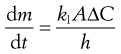
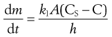
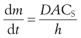
An equation known as the Noyes–Whitney equation was developed to define the dissolution from a single spherical particle. This equation has found great usefulness in the estimation or prediction of the dissolution rate of pharmaceutical particles. The rate of mass transfer of solute molecules or ions through a static diffusion layer (dm/dt) is directly proportional to the area available for molecular or ionic migration (A), the concentration difference (ΔC) across the boundary layer and is inversely proportional to the thickness of the boundary layer (h).
This relationship is shown in Equation 2.3 and in a slightly modified form in Equation 2.4.
 (2.3)
(2.3)
 (2.4)
(2.4)
The constant k1 is known as the diffusion coefficient. It is commonly given the symbol D and has the units of m2/s.
If the volume of the solvent is large, or solute is removed from the bulk of the dissolution medium by some process at a faster rate than it passes into solution, then C remains close to zero and the term (CS – C) in Equation 2.4 may be approximated to CS. In practice, if the volume of the dissolution medium is so large that C is not allowed to exceed 10% of the value of CS, then the same approximation may be made. In either of these circumstances dissolution is said to occur under ‘sink’ conditions and Equation 2.4 may be simplified to:
 (2.5)
(2.5)
Sink conditions may arise in vivo when a drug is absorbed into the body from its solution in the gastrointestinal fluids at a faster rate than it dissolves in those fluids from a solid dosage form, such as a tablet. The phrase is illustrative of the solute molecules ‘disappearing down a sink’!
If solute is allowed to accumulate in the dissolution medium to such an extent that the above approximation is no longer valid, i.e. when C > (CS/10), then ‘non-sink’ conditions are said to be in operation. When C builds up to such an extent that it equals CS, i.e. the dissolution medium is saturated with solute, it is clear from Equation 2.4 that the overall rate of dissolution will be zero.
Factors affecting the rate of dissolution
The various factors that affect the in vitro rate of diffusion-controlled dissolution of solids into liquids can be predicted by examination of the Noyes–Whitney equation (Eqns 2.3 or 2.4). Most of the effects of these factors are included in the summary given in Table 2.1.
Table 2.1
Factors affecting in-vitro dissolution rates of solids in liquids
| Term in Noyes–Whitney equation (Eqn 2.4) | Affected by |
| A: surface area of undissolved solid (Rate of dissolution increases proportionally with increasing A) |
Size of solid particles (A increases with particle size reduction) Dispersibility of powdered solid in dissolution medium Porosity of solid particles |
| CS: saturated solubility of solid in dissolution medium (Rate of dissolution increases proportionally with increasing difference between CS and C. Thus high CS speeds up dissolution rate) |
Temperature Nature of dissolution medium Molecular structure of solute Crystalline form of solid Presence of other compounds |
| C: concentration of solute in solution at time t (Rate of dissolution increases proportionally with increasing difference between CS and C. Thus low C speeds up dissolution rate) |
Volume of dissolution medium (increased volume decreases C) Any process that removes dissolved solute from the dissolution medium (hence decreasing C) |
| k: dissolution rate constant | Diffusion coefficient D of solute in the dissolution medium Viscosity of medium |
| h: thickness of boundary layer (Rate of dissolution decreases proportionally with increasing boundary layer thickness) |
Degree of agitation of dissolution medium (increased agitation decreases boundary layer thickness). |
Clearly, increases in those factors on the top of the right-hand side of the Noyes–Whitney equation will increase the rate of diffusion (and therefore rate of dissolution) and increases in factors at the bottom of the equation will result in a decreased rate of dissolution. The opposite situation obviously applies regarding a reduction in these parameters. Each of these is discussed briefly below.
Surface area of undissolved solid (A)
Size of solid particles.
The surface area of isodiametric particles is inversely proportional to their particle size. Much practical evidence exists to show that, in general, milling or other means of particle size reduction will increase the rate of dissolution of sparingly soluble drugs. An added complication is that particle size will change during the dissolution process, because large particles will become smaller and small particles will eventually disappear. This effect is shown in Figure 2.4.
Compacted masses of solid may also disintegrate into smaller particles, thus increasing the surface area available for dissolution as the disintegration process progresses. (This effect is shown in Figure 30.7 and explained further in the associated discussion.)
Dispersibility of powdered solid in dissolution medium.
If solid particles form cohered masses in the dissolution medium, then the surface area available for dissolution is reduced. This effect may be overcome by the addition of a wetting agent to improve the dispersion of the solid into primary powder particles.
Porosity of solid particles.
Pores in some materials, particularly granulated ones, may be large enough to allow access of the dissolution medium and outward diffusion of dissolved solute molecules.
Solubility of solid in dissolution medium (CS)
Temperature.
Dissolution may be an exothermic or an endothermic process and so temperature changes will influence the energy balance and thus the energy available to promote dissolution.
Nature of dissolution medium.
Factors such as solubility parameters, pH and presence of cosolvents will affect the rate of dissolution.
Molecular structure of solute.
Factors such as the use of salts of either weakly acidic or weakly basic drugs, or esterification of neutral compounds, can influence solubility and dissolution rate.
Crystalline form of solid.
The presence of polymorphs, hydrates, solvates or the amorphous form of the drug can all have an influence on dissolution rate.
Presence of other compounds.
The common-ion effect, complex formation and the presence of solubilizing agents can affect the rate of dissolution.
Concentration of solute in solution at time t (C)
Volume of dissolution medium.
If the volume of the dissolution medium is small, C can rapidly increase during dissolution and approach CS. If the volume is large, then C may be negligible with respect to CS and thus ‘sink’ conditions will operate. This can be controlled in vitro but must be taken into account in vivo as the volume of the stomach contents can vary greatly (hence the common instruction ‘To be taken with a glass of water’). Also, the volume of the fluid in the rectum and vagina is small (see Chapter 42) and so this consideration can be important in drug delivery from suppositories and pessaries.
Any process that removes dissolved solute from the dissolution medium.
For example, adsorption on to an insoluble adsorbent, partitioning into a second liquid that is immiscible with the dissolution medium, removal of solute by dialysis or by continuous replacement of solution by fresh dissolution medium can result in a decrease in C and thus an increased rate of dissolution.
Dissolution rate constant (k)
Thickness of the boundary layer.
This is affected by the degree of agitation, which in turn depends on the speed of stirring or shaking, shape, size and position of stirrer, volume of dissolution medium, shape and size of container, and viscosity of dissolution medium.
Diffusion coefficient of solute in the dissolution medium.
The diffusion coefficient of solute in the dissolution medium is affected by the viscosity of the dissolution medium, and the molecular characteristics and size of diffusing molecules.
It should be borne in mind that pharmaceutical scientists are often concerned with the rate of dissolution of a drug from a formulated product such as a tablet or a capsule, as well as with the dissolution rates of pure solids. In practice, the rate of dissolution can have either zero-order, first-order, second-order or cube-root kinetics. These are discussed later in the book when relevant to particular dosage forms. Later chapters in this book can also be consulted for information on the influence of formulation factors on the rates of release of drugs into solution from various dosage forms.
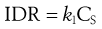
Intrinsic dissolution rate
Since the rate of dissolution is dependent on so many factors, it is advantageous to have a measure of the rate of dissolution which is independent of some of these – rate of agitation and area of solute available in particular. In the latter case, this will change greatly in a conventional tablet formulation as the tablet breaks up into granules and then into primary powder particles as it comes in contact with water.
A useful parameter is the intrinsic dissolution rate (IDR). IDR is the rate of mass transfer per area of dissolving surface and typically has the units of mg mm−2 s−1. IDR should be independent of boundary layer thickness and volume of solvent (i.e. it is assumed that sink conditions have been achieved). IDR is given by:
 (2.6)
(2.6)
Thus, IDR measures the intrinsic properties of the drug only as a function of the dissolution media, e.g. its pH, ionic strength, presence of counter ions, etc., and is independent of many other factors.
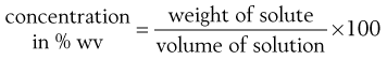
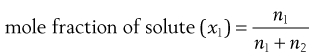
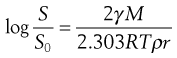
Techniques for measuring IDR
Rotating and static disc methods are used. In these methods, the compound to be assessed for rate of dissolution is compacted into a non-disintegrating disc. This is mounted in a holder so that only one face of the disc is exposed to the dissolution medium (Fig. 2.5). The holder and disc are immersed in the dissolution medium and either held in a fixed position in the static disc method or rotated at a given speed in the rotating disc method. Samples of dissolution medium are removed after known times, filtered and assayed. Further information on this methodology can be found in Chapter 23.
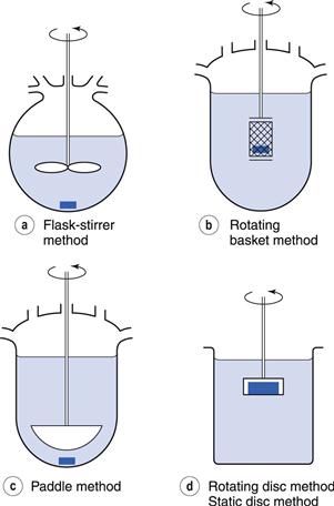
This design of test attempts to ensure that the surface area, from which dissolution can occur, remains constant. Under these conditions, the amount of substance dissolved per unit time and unit surface area can be determined. This is the intrinsic dissolution rate and should be distinguished from the measurements obtained from other methods. In non-disc methods (Chapter 35) the surface area of the drug that is available for dissolution changes considerably during the course of the determination because the dosage form usually disintegrates into many smaller particles and the size of these particles then decreases as dissolution proceeds and, generally, the area of dissolving surface is unknown at any particular time.
Measurement of dissolution rates of drugs from dosage forms
Many methods have been described in the literature, particularly in relation to the determination of the rate of release of drugs into solution from tablet and capsule formulations, because such release may have an important effect on the therapeutic efficacy of these dosage forms (Chapter 20). In-vitro dissolution tests for assessing the dissolution rates of drugs from solid unit dosage forms are discussed fully in Chapter 35. Reference should be made to other chapters in this book for information on the dissolution methods applied to other specific dosage forms.
Solubility
The solution produced when equilibrium is established between undissolved and dissolved solute in a dissolution process is termed a saturated solution. The amount of substance that passes into solution in order to establish this equilibrium at constant temperature and so produce a saturated solution is known as the solubility of the substance. It is possible to obtain supersaturated solutions but these are unstable and precipitation of the excess solute tends to occur readily and spontaneously.
Methods of expressing solubility and concentration
Solubilities may be expressed by any of the variety of concentration terms explained below. In general, solubility is expressed in terms of the maximum mass or volume of solute that will dissolve in a given mass or volume of solvent at a particular temperature and at equilibrium.
Expressions of concentration
Quantity per quantity
Concentrations are often expressed simply as the weight or volume of solute that is contained in a given weight or volume of the solution. The majority of solutions encountered in pharmaceutical practice consist of solids dissolved in liquids. Consequently, concentration is expressed most commonly by the weight of solute contained in a given volume of solution. Although the SI unit is kg m−3 the terms that are used in practice are based on more convenient or appropriate weights and volumes. For example, in the case of a solution with a concentration of 1 kg m−3 the strength may be denoted by any one of the following concentration terms, depending on the circumstances:
1 g L−1, 0.1 g per 100 mL, 1 mg mL−1, 5 mg in 5 mL or 1 µg µL−1.
Percentage
Pharmaceutical scientists have a preference for quoting concentrations in percentages. The concentration of a solution of a solid in a liquid is given by:
 (2.7)
(2.7)
Equivalent percentages based on weight (w) and volume (v) ratios (expressed as % v/w, % v/v and % w/w) can also be used for solutions of liquids in liquids and solutions of gases in liquids.
It should be realized that if concentration is expressed in terms of weight of solute in a given volume of solution then changes in volume caused by temperature fluctuations will alter the concentration.
Parts
Pharmacopoeias give information on the approximate solubility of official substances in terms of the number of ‘parts’ of solute dissolved in a stated number of ‘parts’ of solution. Use of this method to describe the concentration of a solution of a solid in a liquid suggests that a certain number of parts by weight (g) of solid are contained in a given number of parts by volume (mL) of solution. In the case of solutions of liquids in liquids, parts by volume of solute in parts by volume of solution are intended, whereas with solutions of gases in liquids, parts by weight of gas in parts by weight of solution are inferred. The use of ‘parts’ in scientific work, or indeed in practice, is not recommended as there is the chance for some degree of ambiguity.
Molarity
This is the number of moles of solute contained in 1 dm3 (or more commonly expressed in pharmaceutical science as 1 litre) of solution. Thus, solutions of equal molarity contain the same number of solute molecules in a given volume of solution. The unit of molarity (M) is mol L−1 (equivalent to 103 mol m−3 if converted to the strict SI unit).
Molality
This is the number of moles of solute divided by the mass of the solvent, i.e. its SI unit is mol kg−1. Although it is less likely to be encountered in pharmaceutical science than the other terms, it does offer a more precise description of concentration because it is unaffected by temperature.
Mole fraction
This is often used in theoretical considerations and is defined as the number of moles of solute divided by the total number of moles of solute and solvent, i.e.:
 (2.8)
(2.8)
where n1 and n2 are the numbers of moles of solute and solvent, respectively.
Milliequivalents and normal solutions
The concentrations of solutes in body fluids and in solutions used as replacements for these fluids are usually expressed in terms of the number of millimoles (1 millimole = one-thousandth of a mole) in a litre of solution. In the case of electrolytes, however, these concentrations may still be expressed in terms of milliequivalents per litre. A milliequivalent (mEq) of an ion is, in fact, one-thousandth of the gram equivalent of the ion, which is, in turn, the ionic weight expressed in grams divided by the valency of the ion. Alternatively:
 (2.9)
(2.9)
Knowledge of the concept of chemical equivalents is also required in order to understand the use of ‘normality’ as a means of expressing the concentration of solutions. A normal solution, i.e. one with a concentration of 1 N, is one that contains the equivalent weight of the solute, expressed in grams, in 1 litre of solution. It was expected that this term would have disappeared following the introduction of SI units but it is still encountered in some volumetric assay procedures.
Qualitative descriptions of solubility
Pharmacopoeias also express approximate solubilities that correspond to descriptive terms such as ‘freely soluble’ and ‘sparingly soluble’. The interrelationship between such terms and approximate solubility is shown in Table 2.2.
Table 2.2
Descriptive solubility: USP and PhEur terms for describing solubility
| Descriptive term | Parts solvent to 1 part solute (approximate weight of solvent (g) necessary to dissolve 1 g of solute) | Solubility range (mg mL−1) |
| Very soluble | Less than 1 | ≥ 1000 |
| Freely soluble | 1–10 | 100–1000 |
| Soluble | 10–30 | 33–100 |
| Sparingly soluble | 30–100 | 10–33 |
| Slightly soluble | 100–1000 | 1–10 |
| Very slightly soluble | 1000–10 000 | 0.1–1 |
| Practically insoluble* | More than 10 000 | ≤0.1 |
*This term is absent from the PhEur.
Prediction of solubility
Probably the most sought after information about solutions in formulation problems is ‘what is the best solvent for a given solute?’. Theoretical prediction of precise solubility is an involved and occasionally unsuccessful operation but, from knowledge of the structure and properties of solute and solvent, an educated guess is possible. This guess is best expressed in subjective terms, such as ‘very soluble’ or ‘sparingly soluble’, as described above. Often (particularly in pre- or early formulation) this is all the information that the formulator requires. A more precise value can be obtained later in the development process.
Speculation on what is likely to be a good solvent is usually based on the ‘like dissolves like’ principle. That is, a solute dissolves best in a solvent with similar chemical properties. The concept traditionally follows two rules:
Chemical groups that confer polarity to their parent molecules are known as polar groups. In the context of solubility, a polar molecule has a high dipole moment.
To rationalize the above rules, you can consider the forces of attraction between solute and solvent molecules. The following explains the basic physicochemical properties of solutions that lead to such observations.
Physicochemical prediction of solubility
Similar types of intermolecular force may contribute to solute–solvent, solute–solute and solvent–solvent interactions. The attractive forces exerted between polar molecules are much stronger, however, than those that exist between polar and non-polar molecules or between non-polar molecules themselves. Consequently, a polar solute will dissolve to a greater extent in a polar solvent, where the strength of the solute/solvent interaction will be comparable to that between solute molecules, than in a non-polar solvent, where the solute/solvent interaction will be relatively weak. In addition, the forces of attraction between the molecules of a polar solvent will be too great to facilitate the separation of these molecules by the insertion of a non-polar solute between them, because the solute–solvent forces will again be relatively weak. Thus, solvents for non-polar solutes tend to be restricted to non-polar liquids.
The above considerations thus follow the very general ‘like dissolves like’ principle, i.e. a polar substance will dissolve in a polar solvent and a non-polar substance will dissolve in a non-polar solvent. Such generalizations should be treated with caution, because the intermolecular forces involved in the process of dissolution are influenced by factors that are not obvious from a consideration of the overall polarity of a molecule. For example, the possibility of intermolecular hydrogen bond formation between solute and solvent may be more significant than polarity.
Solubility parameters.
Attempts have been made to define a parameter that indicates the ability of a liquid to act as a solvent. The most satisfactory approach, introduced by Hildebrand & Scott in 1962, is based on the concept that the solvent power of a liquid is influenced by its intermolecular cohesive forces and that the strength of these forces can be expressed in terms of a solubility parameter. The initial parameters, which are concerned with the behaviour of non-polar, non-interacting liquids, are referred to as Hildebrand solubility parameters. Whilst these provide good quantitative predictions of the behaviour of a small number of hydrocarbons, they only provide a broad qualitative description of the behaviours of most liquids, because of the influence of factors such as hydrogen bond formation and ionization. The concept has been extended, however, by the introduction of partial solubility parameters, e.g. Hansen parameters and interaction parameters. These have improved the quantitative treatment of systems in which polar effects and interactions occur.
Solubility parameters, in conjunction with the electrostatic properties of liquids, e.g. dielectric constant and dipole moment, have often been linked by empirical or semi-empirical relationships either to these parameters or to solvent properties. Studies on solubility parameters are reported in the pharmaceutical literature. The use of dielectric constants as indicators of solvent power has also received attention but deviations from the behaviour predicted by such methods may occur in practice.
Mixtures of liquids are often used as solvents. If the two liquids have similar chemical structures, e.g. benzene and toluene, then neither tends to associate in the presence of the other and the solvent properties of a 50 : 50 mixture would be the mean of those of each pure liquid. If the liquids have dissimilar structures, e.g. water and propanol, then the molecules of one of them tend to associate with each other and so form regions of high concentration within the mixture. The solvent properties of this type of system are not so simply related to its composition as in the previous case.
Solubility of solids in liquids
Solutions of solids in liquids are the most common type of solution encountered in pharmaceutical practice. A pharmaceutical scientist should therefore be aware of the general method of determining the solubility of a solid in a liquid and the various precautions that should be taken during such determinations.
Determination of the solubility of a solid in a liquid
The following points should be observed in all solubility determinations:
• The solvent and solute must be as pure as possible. The presence of small amounts of many impurities may either increase or decrease the measured solubility. This is a particular problem with early preformulation samples which are often impure, and here special care must be taken (discussed further in Chapter 23).
• A saturated solution must be obtained before any solution is removed for analysis and then all undissolved material removed prior to analysis.
• The method of separating a sample of saturated solution from undissolved solute must be satisfactory.
• The method of analysing the solution must be sufficiently accurate and reliable.
A saturated solution is obtained either by stirring excess powdered solute with solvent for several hours at the required temperature, until equilibrium has been attained, or by warming the solvent with an excess of the solute and allowing the mixture to cool to the required temperature. It is essential that some undissolved solid should be present at the completion of the cooling stage in order to ensure that the solution is saturated and neither subsaturated or supersaturated.
A sample of the saturated solution is obtained for analysis by separating out undissolved solid from the solution. Filtration is usually used, but precautions should be taken to ensure that:
• it is carried out at the temperature of the solubility determination in order to prevent any change in the equilibrium between dissolved and undissolved solute
• loss of any volatile component does not occur
• adsorption of sample material onto surfaces within the filter is minimized.
Membrane filters that can be used in conjunction with conventional syringes fitted with suitable in-line adapters have proved to be successful.
The amount of solute contained in the sample of saturated solution may be determined by a variety of methods, e.g. gravimetric analysis, UV spectrophotometry and chromatographic methods (particularly HPLC). The selection of an appropriate method is affected by the nature of the solute and the solvent and by the concentration of the solution.
Factors affecting the solubility of solids in liquids
Knowledge of these factors, together with their practical applications, as discussed below, is an important aspect of a pharmaceutical scientist’s expertise. Additional information, which shows how some of these factors may be used to improve the solubility and bioavailability of drugs, is given in Chapters 24 and 20, respectively.
Temperature.
The dissolution process is usually an endothermic one, i.e. heat is normally absorbed when dissolution occurs. In this type of system, supply of heat and a rise in temperature will lead to an increase in the solubility of a solid that has a positive heat of solution. Conversely, in the case of the less commonly occurring systems that exhibit exothermic dissolution, then an increase in temperature will result in a decrease in solubility.
Plots of solubility versus temperature, referred to as solubility curves, are often used to describe the effect of temperature on a given system. Some examples are shown in Figure 2.6. Most of the curves are continuous. However, abrupt changes in slope may be observed with some systems if a change in the nature of the dissolving solid occurs at a specific transition temperature. For example, sodium sulfate exists as the decahydrate Na2SO4.10H2O up to 32.5°C and its dissolution in water is an endothermic process. Its solubility therefore increases with a rise in temperature until 32.5 °C is reached. Above this temperature the solid is converted into the anhydrous form (Na2SO4) and the dissolution of this compound is exothermic. The solubility therefore exhibits a change from a positive to a negative slope as the temperature exceeds the transition value.

Molecular structure of solute.
It should be appreciated from the previous comments in this chapter on the prediction of solubility that the nature of the solute and the solvent will be of paramount importance in determining the solubility of a solid in a liquid. It should also be realized that even a small change in the molecular structure of a compound can have a marked effect on its solubility in a given liquid. For example, the introduction of a hydrophilic hydroxyl group can produce a large improvement in water solubility as evidenced by the more than 100-fold difference in the solubility of phenol compared with benzene.
In addition, the conversion of a weak acid to its sodium salt leads to a much greater degree of ionic dissociation of the compound when it dissolves in water. The overall interaction between solute and solvent is increased markedly and the solubility consequently rises. An example of this effect is provided by a comparison of the aqueous solubility of salicylic acid and that of its sodium salt, which are 1 in 550 and 1 in 1, respectively.
The reduction in aqueous solubility of a parent drug by its esterification may also be cited as an example of the effects of changes in the chemical structure of the solute. Such a reduction in solubility may be beneficial to provide a suitable method for:
• masking the taste of a parent drug. For example, chloramphenicol palmitate has been used in paediatric suspensions rather than the more soluble and very bitter tasting chloramphenicol base
• protecting the parent drug from excessive degradation in the gut, e.g. erythromycin propionate is less soluble and consequently less readily degraded than erythromycin
• increasing the ease of absorption of drugs from the gastrointestinal tract, e.g. erythromycin propionate is also more readily absorbed than erythromycin.
Nature of solvent: cosolvents.
The importance of the nature of the solvent has already been discussed in terms of the statement ‘like dissolves like’ and in relation to solubility parameters. In addition, the point has been made that mixtures of solvents may be employed. Such mixtures are often used in pharmaceutical practice in order to obtain aqueous-based systems that contain solutes in excess of their individual solubility in pure water. This is achieved by using cosolvents such as ethanol or propylene glycol, which are miscible with water and which act as better solvents for the solute in question.
For example, the aqueous solubility of metronidazole is about 100 mg in 10 mL. The solubility of this drug can be increased markedly by the incorporation of one or more water-miscible cosolvents so that a solution containing 500 mg in 10 mL (and thus suitable for parenteral administration in the treatment of anaerobic infections) can be obtained.
Crystal characteristics: polymorphism and solvation.
When the conditions under which crystallization is allowed to occur are varied, some substances produce crystals in which the constituent molecules are aligned in different ways with respect to one another in the lattice structure. These different crystalline forms of the same substance, which are known as polymorphs, consequently possess different lattice energies and this difference is reflected by changes in other properties. For example, the polymorphic form with the lowest free energy will be the most stable and possess the highest melting point. Other less stable (or metastable) forms will tend to transform into the most stable one at rates that depend on the energy differences between the metastable and stable forms.
Many drugs exhibit polymorphism, e.g. steroid and sulfonamide polymorphs are common. Polymorphs are explained more fully in Chapters 8 and 23, which also includes an explanation of why polymorphs may have different solubilities. Examples of the importance of polymorphism with respect to the bioavailability of drugs are given in Chapter 20.
The effect of polymorphism on solubility is particularly important from a pharmaceutical point of view, because it provides a means of increasing the solubility of a crystalline material, and hence its rate of dissolution, by using a metastable polymorph.
Although the more soluble polymorphs are metastable and will convert to the stable form, the rate of such conversion is often slow enough for the metastable form to be regarded as being sufficiently stable from a pharmaceutical point of view. The degree of conversion should obviously be monitored during storage of the drug product to ensure that its efficacy is not altered significantly. There are products on the market containing a more soluble, but less stable, polymorph of the drug, where the chosen polymorph is stable enough to survive the approved storage conditions and shelf-life.
Conversion to the less soluble and most stable polymorph may contribute to the growth of crystals in suspension formulations. Examples of the importance of polymorphism with respect to the occurrence of crystal growth in suspensions are given in Chapter 26.
The absence of a crystalline structure that is usually associated with an amorphous powder (discussed in Chapter 8) may also lead to an increase in the solubility of a drug when compared with that of its crystalline form.
In addition to the effect of polymorphism, the lattice structures of crystalline materials may be altered by the incorporation of molecules of the solvent from which crystallization occurred (discussed in Chapter 8). The resultant solids are called solvates and the phenomenon is referred to correctly as solvation and sometimes incorrectly and confusingly as pseudopolymorphism. The alteration in crystal structure that accompanies solvation will affect the internal energetics of the solid so that the solubility of the solvated and unsolvated crystals will differ.
If water is the solvating molecule, i.e. a hydrate is formed, then the interaction between the substance and water that occurs in the crystal phase reduces the amount of energy liberated when the solid hydrate dissolves in water. Consequently, hydrated crystals tend to exhibit a lower aqueous solubility than their unhydrated forms. This decrease in solubility can lead to precipitation of drugs from solutions.
In contrast, the aqueous solubility of other, i.e. non-aqueous, solvates is often greater than those of the unsolvated forms. Examples of the effects of solvation and the attendant changes in solubilities of drugs on their bioavailabilities are given in Chapter 20.
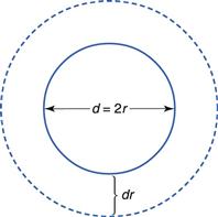
Particle size of the solid.
The changes in interfacial free energy that accompany the dissolution of particles of varying sizes cause the solubility of a substance to increase with decreasing particle size, as indicated by Equation 2.10.
 (2.10)
where S is the solubility of small particles of radius r, So is the normal solubility (i.e. of a solid consisting of fairly large particles), γ is the interfacial energy, M is the molecular weight of the solid, ρ is the density of the bulk solid, R is the gas constant and T is the thermodynamic temperature.
The increase in solubility with decrease in particle size ceases when the particles have a very small radius (less than about 1 µm), and any further decrease in size can cause a decrease in solubility. It has been postulated that this change arises from the presence of an electrical charge on the particles and that the effect of this charge becomes more important as the particle size decreases. Such solubility changes are rarely a problem in conventional dosage forms and drug delivery but could be significant with nanotechnology products.
pH.
If the pH of a solution of either a weakly acidic drug or a salt of such a drug is reduced,then the proportion of unionized acid molecules in the solution increases. Precipitation may occur, therefore, because the solubility of the unionized species is less than that of the ionized form. Conversely, in the case of solutions of weakly basic drugs or their salts, precipitation is favoured by an increase in pH. Such precipitation is an example of one type of chemical incompatibility that may be encountered in the formulation of liquid medicines.
This relationship between pH and solubility of ionized solutes is extremely important with respect to the ionization of weakly acidic and basic drugs as they pass through the gastrointestinal tract and can experience pH changes between about 1 and 8. This will affect the degree of ionization of the drug molecules which in turn influences their solubility and their ability to be absorbed. This aspect is discussed elsewhere in this book in some detail and the reader is referred in particular to Chapters 3 and 20.
The relationship between pH, pKa and solubility of weakly acidic or weakly basic drugs is given by a modification of the Henderson–Hasselbalch equation. To avoid repetition here, the reader is referred to the relevant section of Chapter 3.
Common ion effect.
The equilibrium in a saturated solution of a sparingly soluble salt in contact with undissolved solid may be represented by:
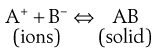 (2.11)
From the Law of Mass Action:
 (2.12)
where the square brackets signify concentrations of the respective components and thus the equilibrium constant K for this reversible reaction is given by Equation 2.13:
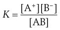 (2.13)
Since the concentration of a solid may be regarded as being constant then this may be written as:
 (2.14)
where  is a constant known as the solubility product of compound AB.
If each molecule of the salt contains more than one ion of each type, e.g. 
 , then in the definition of the solubility product, the concentration of each ion is expressed to the appropriate power, i.e.:
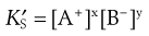 (2.15)
These equations for the solubility product are applicable only to solutions of sparingly soluble salts.
The presence of additional A+ in the dissolution medium, i.e. where A+ is a common ion, would push the equilibrium shown in Equation 2.11 towards the left in order to restore the equilibrium. Solid AB will be precipitated and the solubility of this compound is therefore decreased. This is known as the common ion effect. The addition of common B− ions would have the same effect. An example is the reduced solubility of a hydrochloride salt of a drug in the stomach.
The precipitating effect of the presence of ions and other ingredients in the dissolution medium (as may be encountered in the gastrointestinal tract, for example) is often less apparent in practice than expected from the above discussion. The reasons for this are explained in the following sections:
Effect of different electrolytes on the solubility product.
The solubility of a sparingly soluble electrolyte may be increased by the addition of a second electrolyte that does not possess ions common to the first, i.e. it is a different electrolyte.
Effective concentration of ions.
The activity of a particular ion is related to its effective concentration. In general, this is a lower than the actual concentration because some ions produced by dissociation of the electrolyte are strongly associated with other oppositely charged ions and do not contribute so effectively to the properties of the system as completely unallocated ions.
Effect of non-electrolytes on the solubility of electrolytes.
The solubility of electrolytes depends on the dissociation of dissolved molecules into ions. This dissociation is affected by the dielectric constant of the solvent, which is a measure of the polar nature of the solvent. Liquids with a high dielectric constant (e.g. water) are able to reduce the attractive forces that operate between oppositely charged ions produced by dissociation of an electrolyte.
If a water-soluble non-electrolyte, such as alcohol, is added to an aqueous solution of a sparingly soluble electrolyte, the solubility of the latter is decreased because the alcohol lowers the dielectric constant of the solvent and ionic dissociation of the electrolyte becomes more difficult.
Effect of electrolytes on the solubility of non-electrolytes.
Non-electrolytes do not dissociate into ions in aqueous solution, and in dilute solution the dissolved species therefore consists of single molecules. Their solubility in water depends on the formation of weak inter-molecular bonds (hydrogen bonds) between their molecules and those of water. The presence of a very soluble electrolyte, the ions of which have a marked affinity for water, will reduce the solubility of a non-electrolyte by competing for the aqueous solvent and breaking the inter-molecular bonds between the non-electrolyte and water. This effect is important in the precipitation of proteins.
Complex formation.
The apparent solubility of a solute in a particular liquid may be increased or decreased by the addition of a third substance which forms an intermolecular complex with the solute. The solubility of the complex will determine the apparent change in the solubility of the original solute.
Solubilizing agents.
These agents are capable of forming large aggregates or micelles in solution when their concentrations exceed certain values. In aqueous solution the centre of these aggregates resembles a separate organic phase and organic solutes may be taken up by the aggregates, thus producing an apparent increase in their solubility in water. This phenomenon is known as solubilization. A similar phenomenon occurs in organic solvents containing dissolved solubilizing agents because the centre of the aggregates in these systems constitutes a more polar region than the bulk of the organic solvent. If polar solutes are taken up into these regions, their apparent solubility in the organic solvents is increased.
Solubility of gases in liquids
The amount of gas that will dissolve in a liquid is determined by the nature of the two components and by temperature and pressure.
Provided that no reaction occurs between the gas and liquid then the effect of pressure is indicated by Henry’s Law which states that at constant temperature, the solubility of a gas in a liquid is directly proportional to the pressure of the gas above the liquid. The law may be expressed by Equation 2.16:
 (2.16)
where w is the mass of gas dissolved by unit volume of solvent at an equilibrium pressure p and k is a proportionality constant. Although Henry’s Law is most applicable at high temperatures and low pressures, when solubility is low, it provides a satisfactory description of the behaviour of most systems at normal temperatures and reasonable pressures, unless solubility is very high or reaction occurs. Equation 2.16 also applies to the solubility of each gas in a solution of several gases in the same liquid provided that p represents the partial pressure of a particular gas.
The solubility of most gases in liquids decreases as the temperature rises. This provides a means of removing dissolved gases. For example, water for injections free from either carbon dioxide or air may be prepared by boiling water with minimum exposure to air and prevention of access of air during cooling. The presence of electrolytes may also decrease the solubility of a gas in water by a ‘salting out’ process, which is caused by the marked attraction exerted between electrolyte and water.
Solubility of liquids in liquids
The components of an ideal solution are miscible in all proportions. Such complete miscibility is also observed in some real binary systems, e.g. ethanol and water, under normal conditions. However, if one of the components tends to self-associate because the attractions between its own molecules are greater than those between its molecules and those of the other component, i.e. if a positive deviation from Raoult’s Law occurs, the miscibility of the components may be reduced (Raoult’s Law is discussed more fully in Chapter 3). The extent of the reduction in miscibility depends on the strength of the self-association and, therefore, on the degree of deviation from Raoult’s Law. Thus, partial miscibility may be observed in some systems whereas virtual immiscibility may be exhibited when the self-association is very strong and the positive deviation from Raoult’s Law is large.
In those cases where partial miscibility occurs under normal conditions, the degree of miscibility is usually dependent on the temperature. This dependency is indicated by the phase rule, introduced by J. Willard Gibbs, which is expressed quantitatively by Equation 2.17:
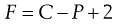 (2.17)
where P and C are the numbers of phases and components in the system, respectively, and F is the number of degrees of freedom, i.e. the number of variable conditions such as temperature, pressure and composition, that must be stated in order to define completely the state of the system at equilibrium.
The overall effect of temperature variation on the degree of miscibility in these systems is usually described by means of phase diagrams, which are graphs of temperature versus composition at constant pressure. For convenience of discussion of their phase diagrams, the partially miscible systems may be divided into the following types.
Systems showing an increase in miscibility with rise in temperature
A positive deviation from Raoult’s Law arises from a difference in the cohesive forces that exist between the molecules of each component in a liquid mixture. This difference becomes more marked as the temperature decreases and the positive deviation may then result in a decrease in miscibility sufficient to cause the separation of the mixture into two phases. Each phase consists of a saturated solution of one component in the other liquid. Such mutually saturated solutions are known as conjugate solutions.
The equilibria that occur in mixtures of partially miscible liquids may be followed either by shaking the two liquids together at constant temperature and analysing samples from each phase after equilibrium has been attained, or by observing the temperature at which known proportions of the two liquids, contained in sealed glass ampoules, become miscible (as indicated by the disappearance of turbidity).
Systems showing a decrease in miscibility with rise in temperature
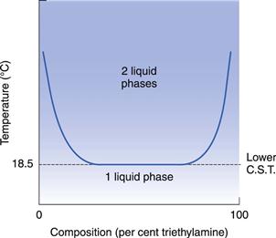
A few mixtures, which probably involve compound formation, exhibit a lower critical solution temperature (CST), e.g. triethylamine plus water and paraldehyde plus water. The formation of a compound produces a negative deviation from Raoult’s Law, and miscibility therefore increases as the temperature falls, as shown in Figure 2.7.
Systems showing upper and lower critical solution temperatures
The decrease in miscibility with increase in temperature in systems having a lower CST is not indefinite. Above a certain temperature, positive deviations from Raoult’s Law become important and miscibility starts to increase again with further rise in temperature. This behaviour produces a closed-phase diagram as shown in Figure 2.8. This behaviour is shown by the nicotine–water system.

Fig. 2.8 Temperature–composition diagram for the nicotine–water system exhibiting upper and lower critical solution temperatures.
In some mixtures where an upper and lower CST are expected, these points are not, in fact, observed since a phase change by one of the components occurs before the relevant CST is reached. For example, the ether–water system should exhibit a lower CST, but water freezes before the temperature is reached.
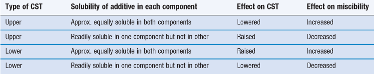
Effects of added substances on critical solution temperatures
CST is an invariant point at constant pressure, but this temperature is very sensitive to impurities or added substances. The effects of additives are summarized in Table 2.3.
Blending
The increase in miscibility of two liquids caused by the addition of a third substance is referred to as blending. The use of propylene glycol as a blending agent, which improves the miscibility of volatile oils and water, can be explained in terms of a ternary-phase diagram. This diagram is a triangular plot which indicates the effects of changes in the relative proportions of the three components at constant temperature and pressure and it presents a good example of the interpretation and use of such phase diagrams.
Distribution of solutes between immiscible liquids
Partition coefficients
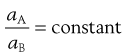
When a substance, which is soluble in both components of a mixture of immiscible liquids, is dissolved in such a mixture, when equilibrium is attained at constant temperature, it is found that the solute is distributed between the two liquids in such a way that the ratio of the activities of the substance in each liquid is a constant. This is known as the Nernst Distribution Law and may be expressed by Equation 2.18:
 (2.18)
where aA and aB are the activities of the solute in solvents A and B, respectively. When the solutions are dilute or when the solute behaves ideally, the activities may be replaced by concentrations (CA and CB):
 (2.19)
The constant K is known as the distribution coefficient or partition coefficient. In the case of sparingly soluble substances, K is approximately equal to the ratio of the solubility (SA and SB) of the solute in each liquid. Thus:
 (2.20)
In most other systems, however, deviation from ideal behaviour invalidates Equation 2.20. For example, if the solute exists as monomers in solvent A and as dimers in solvent B, the distribution coefficient is given by Equation 2.21, in which the square root of the concentration of the dimeric form is used:
 (2.21)
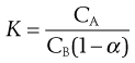
If the dissociation into ions occurs in the aqueous layer, B, of a mixture of immiscible liquids, then the degree of dissociation (α) should be taken into account, as indicated by Equation 2.22:
 (2.22)
The solvents in which the concentrations of the solute are expressed should be indicated when partition coefficients are quoted. For example, a partition coefficient of 2 for a solute distributed between oil and water may also be expressed as a partition coefficient between water and oil of 0.5. This can be represented as 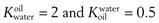 . The abbreviation
  is often used for the former and this notation has become the most commonly used.
Solubility of solids in solids
If two solids are either melted together and then cooled or dissolved in a suitable solvent that is then removed by evaporation, the solid that is redeposited from the melt or the solution will either be a one-phase solid solution or a two-phase eutectic mixture.
In a solid solution, as in other types of solution, the molecules of one component (the solute) are dispersed molecularly throughout the other component (the solvent). Complete miscibility of two solid components is only achieved if:
• the molecular size of the solute is similar to that of the solvent so that a molecule of the former can be substituted for one of the latter in its crystal lattice structure, or
• the solute molecules are much smaller than the solvent molecules so that the former can be accommodated in the spaces of the solvent lattice structure.
These two types of solvent mechanism are referred to as substitution and interstitial effects, respectively. Since these criteria are only satisfied in relatively few systems then it is more common to observe partial miscibility of solids. Thus, dilute solutions of solids in solids may be encountered in systems of pharmaceutical interest; for example, when the solvent is a polymeric material with large spaces between its intertwined molecules that can accommodate solute molecules.
Unlike a solution, a simple eutectic consists of an intimate mixture of the two microcrystalline components in a fixed composition. However, both solid solutions and eutectics provide a means of dispersing a relatively water-insoluble drug in a very fine form, i.e. as molecules or microcrystalline particles, respectively, throughout a water-soluble solid. When the latter carrier solid is dissolved away, the molecules or small crystals of insoluble drug may dissolve more rapidly than a conventional powder because the contact area between drug and water is increased. The rate of dissolution and, consequently, the bioavailability of poorly soluble drugs may be improved, therefore, by the use of solid solutions or eutectics.
Summary
This chapter has shown that the process of dissolution is a change in phase of a molecule or ion. Most often this is from solid to liquid. Simple diffusional mechanisms and equations usually define the rate and extent of this process. The concept of solubility in a pharmaceutical context has also been discussed. The chapter that follows will describe the properties of the solution thus produced.
References
1. Florence AT, Attwood D. Physicochemical Principles of Pharmacy. 5th edn London: Pharmaceutical Press Ltd; 2011.
2. Noyes AA, Whitney WR. The rate of solution of solid substances in their own solutions. Journal of the American Chemical Society. 1897;19:930.
Bibliography
1. Banker GS, Rhodes CT. Modern Pharmaceutics. 4th edn New York: Marcel Dekker; 2002.
2. Barton AFM. Handbook of Solubility Parameters and Other Cohesion Parameters. Boca Raton, Florida: CRC Press; 1991.
3. British Pharmacopoeia (2013). Stationery Office, London.
4. Carstensen JT. Theory of Pharmaceutical Systems, Vol 1 General Principles. London: Academic Press; 1972.
5. European Pharmacopoeia (2013). Council of Europe, Strasburg, France.
6. Hildebrand JH, Prausnitz JM, Scott RL. Regular and Related Solutions: The Solubility of Gases, Liquids and Solids. New York: Van Nostrand Reinhold; 1970.
7. Leeson L, Cartsensen JT. Dissolution Technology. Washington DC: IPT Academy of Pharmaceutical Science; 1974.
8. Price NC, Dwek RA. Principles and Problems in Physical Chemistry for Biochemists. 2nd edn Oxford: Clarendon Press; 1979.
9. Rowe RC, Sheskey PJ, Cook WG, Fenton ME. Handbook of Pharmaceutical Excipients. 7th edn London: The Pharmaceutical Press; 2012.
10. Rowlinson JS, Swinton FL. Liquids and Liquid Mixtures. 3rd edn London: Butterworth Scientific; 1982.
11. Swarbrick J. Drug dissolution and bioavailability. In: Swarbrick J, ed. Current Concepts in the Pharmaceutical Sciences: Biopharmaceutics. Philadelphia: Lea and Febiger; 1970.
12. Troy DB. Remington: The Science and Practice of Pharmacy. 21st edn Maryland, USA: Lippincott, Williams and Wilkins; 2006.
13. United States Pharmacopeia and National Formulary (2012). United States Pharmacopeial Convention, Rockville, Maryland, USA.
14. Wallwork SC, Grant DJW. Physical Chemistry for Students of Pharmacy and Biology. 3rd edn London: Longman; 1977.
15. Wichmann K, Klamt A. Drug solubility and reaction thermodynamics. In: am In: Ende DJ, ed. Chemical Engineering in the Pharmaceutical Industry: R&D to Manufacture. New Jersey: John Wiley & Sons (in conjunction with AIChE); 2010.
16. Williams VR, Mattice WL, Williams HB. Basic Physical Chemistry for the Life Sciences. 3rd edn San Francisco: W. H. Freeman; 1978.