Digital Image Processing
Limitations of Film-Based Imaging
Generic Digital Imaging System
Image Formation and Representation
What is Digital Image Processing?
Characteristics of the Digital Image
LIMITATIONS OF FILM-BASED IMAGING
Film-based imaging has been the workhorse of radiology ever since the discovery of x rays in 1895. Applications of film-based imaging include conventional radiography and tomography, fluoroscopy, and special procedures imaging (angiography, for example). Additionally, nuclear medicine, ultrasound, computed tomography (CT), and magnetic resonance imaging (MRI) use film to record images from which a radiologist can make a diagnosis.
The steps in the production of a film-based radiographic image are very familiar to radiologic technologists. First, the patient is exposed to a predetermined amount of radiation that is needed to provide the required diagnostic image quality. A latent image is formed on the film that is subsequently processed by chemicals in a processor to render the image visible. The processed image is then ready for viewing by a radiologist, who makes a diagnosis of the patient’s medical condition.
The imaging process can also result in poor image quality if the initial radiation exposure has not been accurately determined. For example, if the radiation exposure is too high, the film is overexposed and the processed image appears too dark; thus, the radiologist cannot make a diagnosis from such an image. Alternatively, if the radiation exposure is too low, the processed image appears too light and is not useful to the radiologist. In both these situations the images lack the proper image density and contrast and imaging would have to be repeated to provide an acceptable image quality needed to make a diagnosis. Additionally, the patient would be subjected to increased radiation exposure.
Despite the above problems, film-based imaging has been successful for the past 100 years and it is still being used today in many departments. There are other problems associated with film-based imaging. For example, film is not the ideal vehicle to perform the three basic functions of radiation detection, image display, and image archiving.
As a radiation detector, film-screen cannot show differences in tissue contrast that are less than 10%. This means that film-based imaging is limited in its contrast resolution. The spatial resolution of film-screen systems, however, is the highest of all imaging modalities, and this is the main reason that radiography has played a significant role in imaging patients through the years.
As a display medium, the optical range and contrast for film are fixed and limited. Film can only display once—the optical range and contrast determined by the exposure technique factors used to produce the image. To change the image display (optical range and contrast), another set of exposure technique factors would have to be used, thus increasing the dose to the patient by virtue of a repeat exposure.
As an archive medium, film is usually stored in envelopes and housed in a large room. It thus requires manual handling for archiving and retrieval by an individual.
A digital imaging system and digital image processing can overcome these problems.
GENERIC DIGITAL IMAGING SYSTEM
The major components of a generic digital imaging system for use in radiology are shown in Figure 3-1. These include data acquisition, image processing, image display/storage/archiving, and image communication. As noted in Chapter 1, CT consists of these major components (to be described in detail later in subsequent chapters) and can therefore be classified as a digital imaging system because it uses computers to process images. Each of these components will be described briefly.
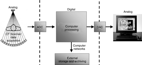
Data Acquisition
The term data acquisition refers to a systematic method of collecting data from the patient. For projection digital radiography and CT, the data are the electron density of the tissues, which is related to the linear attenuation coefficient (μ) of the various tissues. In other words, it is attenuation data that is collected for these imaging modalities. Data acquisition components for these modalities include the x-ray tube and the digital image detectors. The output signal from the detectors is an electrical signal (an analog signal that varies continuously in time). Because a digital computer is used in these imaging systems, the analog signal must be converted into a digital signal (discrete units) for processing by a digital computer. This conversion is performed by an analog-to-digital converter (ADC).
Image Processing
Image processing is performed by a digital computer that takes an input digital image and processes it to produce an output digital image by using the binary number system. Although we typically use the decimal number system (which operates with base 10, that is, 10 different numbers: 0,1,2,3,4,5,6,7,8,9), computers use the binary number system (which operates with base 2, that is, 0 or 1). These two digits are referred to as binary digits or bits. Bits are not continuous but rather they are discrete units. Computers operate with binary numbers, 0 and 1, discrete units that are processed and transformed into other discrete units. To process the word Euclid, it would have to be converted into digital data (binary representation). Thus the binary representation for the word Euclid is 01000101 01010101 01000011 01001100 01001001 01000100.
The ADC sends digital data for digital image processing by a digital computer. Such processing is accomplished by a set of operations and techniques to transform the input image into an output image that suits the needs of the observer (radiologist) to enhance diagnosis. For example, these operations can be used to reduce the noise in the input image, enhance the sharpness of the input image, or change the contrast of the input image. This chapter is concerned primarily with these digital image processing operations and techniques.
Image Display, Storage, and Communication
The output of computer processing, that is, the output digital image, must first be converted into an analog signal before it can be displayed on a monitor for viewing by the observer. Such conversion is the function of the digital-to-analog conversion (DAC). This image can be stored and archived on magnetic data carriers (magnetic tapes/disks) and laser optical disks for retrospective viewing and manipulation. Additionally, these images can be communicated electronically through computer networks to observers at remote sites. In this regard, picture archiving and communication systems (PACS) are becoming commonplace in the modern radiology department.
This chapter explores the fundamentals of digital image processing through a brief history and a description of related topics such as image representation, the digitizing process, image processing operations, and image processing hardware considerations.
HISTORICAL PERSPECTIVES
The history of digital image processing dates to the early 1960s, when the National Aeronautics and Space Administration (NASA) was developing its lunar and planetary exploration program. The Ranger spacecraft returned images of the lunar surface to Earth. These analog images taken by a television camera were converted into digital images and subsequently processed by the digital computer to obtain more information about the moon’s surface.
The development of digital image processing techniques can be attributed to work at NASA’s Jet Propulsion Laboratory at the California Institute of Technology. The technology of digital processing continues to expand rapidly and its applications extend into fields such as astronomy, geology, forestry, agriculture, cartography, military science, and medicine. (An overview of the history of digital image processing technology is shown in Fig. 3-2.) The technology has found widespread applications in medicine and particularly in diagnostic imaging, where it has been successfully applied to ultrasound, digital radiography, nuclear medicine, CT, and MRI (Huang, 2004). Digital image processing is a multidisciplinary subject that includes physics, mathematics, engineering, and computer science.

FIGURE 3-2 Overview of the first 20 years of important developments in digital image processing. Rights were not granted to include this figure in electronic media. Please refer to the printed book. From Green WB: Digital image processing: a systems approach, ed 2, New York, 1989, Van Nostrand Reinhold.
IMAGE FORMATION AND REPRESENTATION
An understanding of images is necessary to define digital image processing. Castleman (1996) has classified images on the basis of their form or method of generation. He used set theory to explain image types. According to this theory, images are a subset of all objects. Within the set of images, there are other subsets such as visible images (e.g., paintings, drawings, or photographs), optical images (e.g., holograms), nonvisible physical images (e.g., temperature, pressure, or elevation maps), and mathematical images (e.g., continuous functions and discrete functions). The sine wave is an example of a continuous function (analog signal), whereas a discrete function represents a digital image, as shown in Figure 3-3. Castleman noted that “only the digital images can be processed by computer.”
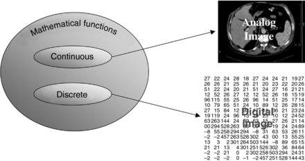
Analog Images
Analog images are continuous images. For example, a black-and-white photograph of a chest x ray is an analog image because it represents a continuous distribution of light intensity as a function of position on the radiograph.
In photography, images are formed when light is focused on film. In radiography, x rays pass through the patient and are projected onto x-ray film. In both cases, films are processed in chemical solutions to render them visible and the images are formed by a photochemical process. Images can also be formed by photoelectronic means, in which the images may be represented as electrical signals (analog signals) that emerge from the photoelectronic device.
Digital Images
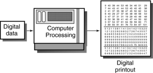
Digital images are numerical representations or images of objects. The formation of digital images requires a digital computer. Any information that enters the computer for processing must first be converted into digital form, or numbers (Fig. 3-4). An important component is the ADC, which converts continuous signals to discrete signals, or digital data (Luiten, 1995).
The computer receives the digital data and performs the necessary processing. The results of this processing are always digital and can be displayed as a digital image (Fig. 3-5).
WHAT IS DIGITAL IMAGE PROCESSING?
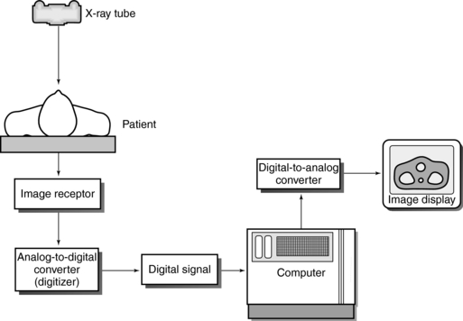
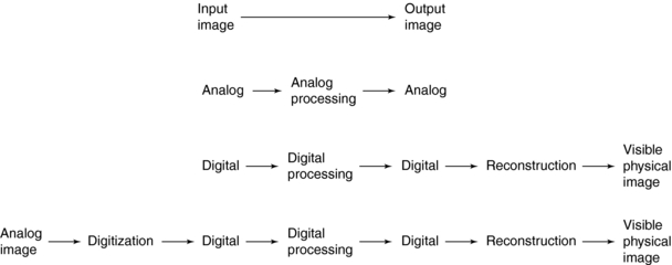
In image processing it is necessary to convert an input image into an output image. If both the input image and output image are analog, this is referred to as analog processing. If both the input image and output image are discrete, this is referred to as digital processing. In cases where an analog image must be converted into digital data for input to the computer, a digitization system is required. CT is based on a reconstruction process whereby a digital image is changed into a visible physical image (Fig. 3-6).
Castleman (1996) defined a process as “a series of actions or operations leading to a desired result; thus, a series of actions or operations are performed upon an object to alter its form in a desired manner.” Castleman also defined digital image processing as “subjecting numerical representations of objects to a series of operations in order to obtain a desired result.”
Given the variety of possible operations (Baxes, 1994), image processing has emerged as a discipline in itself (see box below).
Image Domains
Images can be represented in two domains on the basis of how they are acquired (Huang, 2004). These domains include the spatial location domain and the spatial frequency domain. All images displayed for viewing by humans are in the spatial location domain. Radiography and CT, for example, acquire images in the spatial location domain.
As mentioned earlier, the digital image is a numerical image arranged in such a manner that the location of each number in the image can be identified by using a right-handed x-y coordinate system, where the x-axis describes the rows or lines placed on the image and the y-axis describes the columns, as shown in Figure 3-7. For example, the first pixel in the upper left corner of the image is always identified as 0,0. The spatial location 9,4 will describe a pixel that is located nine pixels to the right of the left-hand side of the image and four lines down from the top of the image. Such an image is said to be in the spatial location domain.
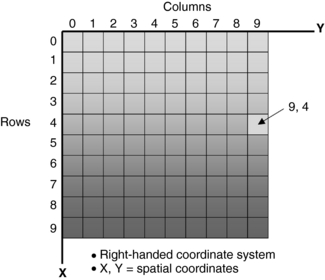
FIGURE 3-7 A right-handed coordinate system used to describe digital images in the spatial location domain. The exact location of a pixel can be found using columns and rows. See text for further explanation.
Images can also be acquired in the spatial frequency domain, such as those acquired in MRI. The term frequency refers to the number of cycles per unit length, that is, the number of times a signal changes per unit length. Although small structures within an object (patient) produce high frequencies that represent the detail in the image, large structures produce low frequencies and represent contrast information in the image.
Digital image processing can transform one image domain into another image domain. For example, an image in the spatial location domain can be transformed into a spatial frequency domain image, as is illustrated in Figure 3-8. The Fourier transform (FT) is used to perform this task. The FT is mathematically rigorous and will not be covered in this article. The FT converts a function in the time domain, (say signal intensity versus time) to a function in frequency domain (say, signal intensity versus frequency). The inverse FT denoted by FT−1 is used to transform an image in the frequency domain back to the spatial location domain for viewing by radiologists and technologists. Physicists and engineers, on the other hand, would probably prefer to view images in the frequency domain.
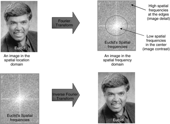
FIGURE 3-8 The Fourier transform is used to convert an image in the spatial location domain into an image in the spatial frequency domain for processing by a computer. The inverse Fourier transform (FT−1) is used to convert the spatial frequency domain image back into a spatial location image for viewing by humans. From Seeram E: Digital image processing, Radiol Technol 75:435-455, 2004. Reproduced by permission of the American Society of Radiologic Technologists.
The major reason for doing this is to facilitate image processing that can enhance or suppress certain features of the image. For example, Huang (2004) points out:
One can use information appearing in the frequency domain, and not easily available in the spatial domain, to detect some inherent characteristics of each type of radiological image. If the image has many edges, there would be many high-frequency components. On the other hand, if the image has only uniform materials, like water or plastic, then it has low-frequency components. On the basis of this frequency in the image, we can selectively change the frequency components to enhance the image. To obtain a smoother appearing image we can increase the amplitude of the low-frequency components, whereas to enhance the edges of bones in the hand x-ray image, we can magnify the amplitude of the high-frequency components.
CHARACTERISTICS OF THE DIGITAL IMAGE
The structure of a digital image can be described with respect to several characteristics or fundamental parameters, including the matrix, pixels, voxels, and the bit depth (Castleman, 1996; Pooley et al, 2001; Seeram and Seeram, 2008; Seibert, 1995).
Matrix
Apart from being a numerical image, there are other elements of a digital image that are important to our understanding of digital image processing. A digital image is made up of a two-dimensional array of numbers, called a matrix. The matrix consists of columns (M) and rows (N) that define small square regions called picture elements, or pixels. The dimension of the image can be described by M, N, and the size of the image is given by the following relationship:

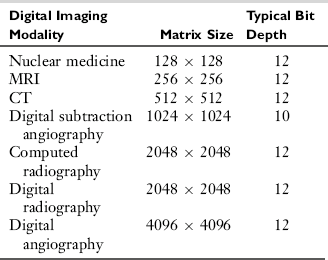
When M = N, the image is square. Generally, diagnostic digital images are rectangular in shape. When imaging a patient with a digital imaging modality, the operator selects the matrix size, sometimes referred to as the field-of-view (FOV). Typical matrix sizes are shown in Table 3-1. It is important to note that as images become larger, they require more processing time and more storage space. Additionally, larger images will take more time to be transmitted to remote locations. In this regard, image compression is needed to facilitate storage and transmission requirements.
Pixels
The pixels that make up the matrix are generally square. Each pixel contains a number (discrete value) that represents a brightness level. The numbers represent tissue characteristics being imaged. For example, in radiography and CT, these numbers are related to the atomic number and mass density of the tissues, and in MRI they represent other characteristics of tissues, such as proton density and relaxation times.
The pixel size can be calculated according to the following relationship:

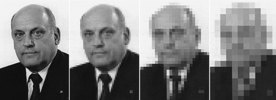
For digital imaging modalities, the larger the matrix size, the smaller the pixel size (for the same FOV) and the better the spatial resolution. The effect of the matrix size on picture clarity can be seen in Figure 3-9.
Voxels
Pixels in a digital image represent the information contained in a volume of tissue in the patient. Such volume is referred to as a voxel (contraction for volume element). Voxel information is converted into numerical values contained in the pixels, and these numbers are assigned brightness levels, as illustrated in Figure 3-10.
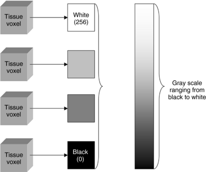
FIGURE 3-10 Voxel information from the patient is converted into numerical values contained in the pixels, and these numbers are assigned brightness levels. The higher numbers represent high signal intensity (from the detectors) and are shaded white (bright) while the low numbers represent low signal intensity, and are shaded dark (black).
Bit Depth
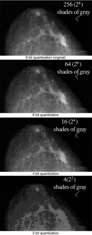
In the relationship M × N × k bits, the term “k bits” implies that every pixel in the digital image matrix M × N is represented by k binary digits. The number of bits per pixel is the bit depth. Because the binary number system uses the base 2, k bits = 2k. Therefore each pixel will have 2k gray levels. For example, in a digital image with a bit depth of 2, each pixel will have 22 (4) gray levels (density). Similarly, a bit depth of 8 implies that each pixel will have 28 (256) gray levels or shades of gray. The effect of bit depth is clearly seen in Figure 3-11. Table 3-1 also provides the typical bit depth for diagnostic digital images.
Effect of Digital Image Parameters on the Appearance of Digital Images
The characteristics of a digital image, that is, the matrix size, the pixel size, and the bit depth, can affect the appearance of the digital image, particularly its spatial resolution and its density resolution.
The matrix size has an effect on the detail or spatial resolution of the image. The larger the matrix size (for the same FOV), the smaller pixel size, hence the better the appearance of detail. Additionally, as the FOV decreases without a change in matrix size, the size of the pixel decreases as well (recall the relationship pixel size = FOV/matrix size), thus improving detail. The operator selects a larger matrix size when imaging larger body parts, such as a chest, to show small details in the anatomy.
The bit depth has an effect on the number of shades of gray, hence the contrast resolution of the image. This is clearly apparent in Figure 3-11.
IMAGE DIGITIZATION
The primary objective during image digitization is to convert an analog image into numerical data for processing by the computer (Seibert, 1995). Digitization consists of three distinct steps: scanning, sampling, and quantization.
Scanning
Consider an image (Fig. 3-12). The first step in digitization is the division of the picture into small regions, or scanning. Each small region of the picture is a picture element, or pixel. Scanning results in a grid characterized by rows and columns. The size of the grid usually depends on the number of pixels on each side of the grid. In Figure 3-12 the grid size is 9 × 9, which results in 81 pixels. The rows and columns identify a particular pixel by providing an address for that pixel. The rows and columns comprise a matrix; in this case, the matrix is 9 × 9. As the number of pixels in the image matrix increases, the image becomes more recognizable and facilitates better perception of image details.
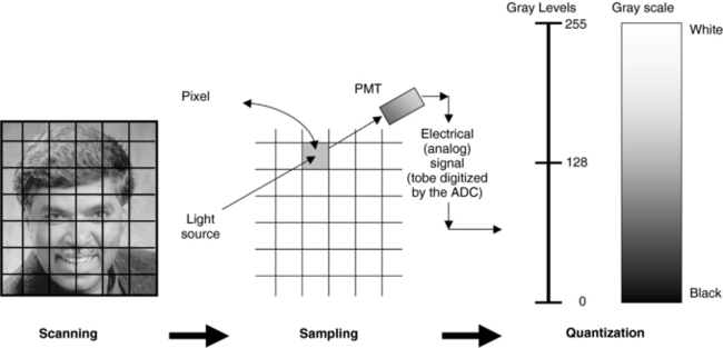
FIGURE 3-12 Three general steps in digitizing an image; scanning, sampling, and quantization. See text for further explanation. Similar steps apply to digital diagnostic techniques. From Seeram E: Digital image processing, Radiol Technol 75: 435-455, 2004. Reproduced by permission of the American Society of Radiologic Technologists.
Sampling
The second step in image digitization is sampling, which measures the brightness of each pixel in the entire image (see Fig. 3-12). A small spot of light is projected onto the transparency and the transmitted light is detected by a photomultiplier tube positioned behind the picture. The output of the photomultiplier tube is an electrical (analog) signal.
Quantization
Quantization is the final step, in which the brightness value of each sampled pixel is assigned an integer (0, or a positive or negative number) called a gray level. The result is a range of numbers or gray levels, each of which has a precise location on the rectangular grid of pixels. The total number of gray levels is called the gray scale, such as eight-level gray scale (see Fig. 3-12). The gray scale is based on the value of the gray levels; 0 represents black and 255 represents white. The numbers in between 0 and 255 represent shades of gray. In the case of two gray levels, the picture would show only black and white. An image can therefore be composed of any number of gray levels, depending on the bit depth.
In quantization, the electrical signal obtained from sampling is assigned an integer that is based on the strength of the signal. In general, the value of the integer is proportional to the signal strength (Seibert, 1995).
The result of the quantization process is a digital image, an array of numbers representing the analog image that was scanned, sampled, and quantized. This array of numbers is sent to the computer for further processing.
Analog-to-Digital Conversion
The conversion of analog signals to digital information is accomplished by the ADC. The ADC samples the analog signal at various times to measure its strength at different points. The more points sampled, the better the representation of the signal. This sampling process is followed by quantization.
Two important characteristics of the ADC are speed and accuracy. Accuracy refers to the sampling of the signal. The more samples taken, the more accurate the representation of the digital image (Fig. 3-13). If enough samples are not taken, the representation of the original signal will be inaccurate after computer processing (Fig. 3-14). This sampling error is referred to as aliasing, and it appears as an artifact on the image. Aliasing artifacts appear as Moiré patterns on the image (Baxes, 1994).
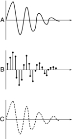
FIGURE 3-13 Good sampling (B) of original analog signal (A) produces an accurate representation of the original signal (C) after computer processing.
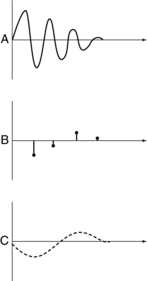
FIGURE 3-14 Poor sampling (B) misrepresents the shape of the original (A) after computer processing (C).
The sampling results in the division of the signal. The more parts to the signal, the greater the accuracy of the ADC. The measurement unit for these parts is the bit. Recall that a bit can be either 0 or 1. In a 1-bit ADC, the signal is divided in two parts (21 = 2). A 2-bit ADC generates four equal parts (22 = 4). An 8-bit ADC generates 256 equal parts (28 = 256). The higher the number of bits, the more accurate the ADC.
The ADC also determines the number of levels or shades of gray represented in the image. A 1-bit ADC results in two integers (0 and 1), which are represented as black and white. A 2-bit ADC results in four numbers, which produce a gray scale with four shades. An 8-bit ADC results in 256 integers (28), ranging from 0 to 255, with 256 shades of gray (see Fig. 3-10).
The other characteristic of the ADC is speed, or the time taken to digitize the analog signal. In the ADC, speed and accuracy are inversely related—that is, the greater the accuracy, the longer it takes to digitize the signal.
Why Digitize Images?
The operations used in digital image processing to transform an input image into an output image to suit the needs of the human observer are several. Baxes (1994) identifies at least five fundamental classes of operations, including image enhancement, image restoration, image analysis, image compression, and image synthesis. Although it is not within the scope of this chapter to describe all of these in any great detail, it is noteworthy to mention the purpose of each of them and state their particular operations. For a more complete and thorough description of these, the interested reader should refer to the work of Baxes (1994).
1. Image enhancement: The purpose of this class of processing is to generate an image that is more pleasing to the observer. Certain characteristics such as contours and shapes can be enhanced to improve the overall quality of the image. The operations include contrast enhancement, edge enhancement, spatial and frequency filtering, image combining, and noise reduction.
2. Image restoration: The purpose of image restoration is to improve the quality of images that have distortions or degradations. Image restoration is commonplace in spacecraft imagery. Images sent to Earth from various camera systems on spacecrafts have distortions/degradations that must be corrected for proper viewing. Blurred images, for example, can be filtered to make them sharper.
3. Image analysis: This class of digital image processing allows measurements and statistics to be performed, as well as image segmentation, feature extraction, and classification of objects. Baxes (1994) indicates that “the process of analyzing objects in an image begins with image segmentation operations, such as image enhancement or restoration operations. These operations are used to isolate and highlight the objects of interest. Then the features of the objects are extracted resulting in object outlines or other object measures. These measures describe and characterize the objects in the image. Finally, the object measures are used to classify the objects into specific categories.” Segmentation operations are used in three-dimensional (3D) medical imaging (Seeram, 2001).
4. Image compression: The purpose of image compression of digital images is to reduce the size of the image to decrease transmission time and reduce storage space. In general, there are two forms of image compression, lossy and lossless compression (Fig. 3-15). In lossless compression there is no loss of any information in the image (detail is not compromised) when the image is decompressed. In lossy compression, there is some loss of image details when the image is decompressed. The latter has specific uses especially in situations when it is not necessary to have exact details of the original image. A more recent form of compression that has been receiving attention in digital diagnostic imaging is that of wavelet (special waveforms) compression. The main advantage of this form of compression is that there is no loss in both spatial and frequency information. Compression has received a good deal of attention in the digital radiology department, including the PACS environment, especially because image data sets are becoming increasingly larger. For this reason it will be described further later in this chapter.
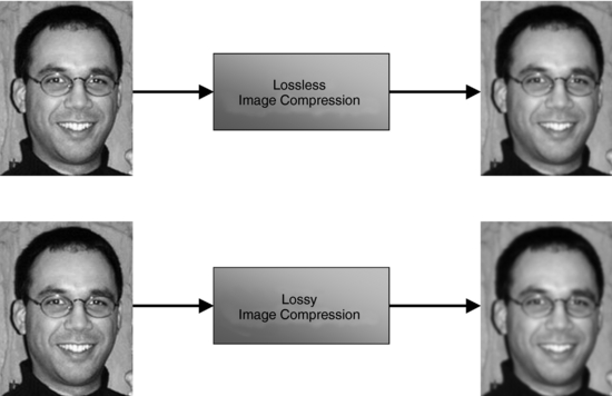
FIGURE 3-15 The effects of two methods of image compression, lossless and lossy, on the quality of the image (visual appearance of the image) of Euclid’s son David, a brilliant, caring, and absolutely wonderful young man. Images courtesy David Seeram.
5. Image synthesis: These processing operations “create images from other images or non-image data. These operations are used when a desired image is either physically impossible or impractical to acquire, or does not exist in a physical form at all” (Baxes, 1994). Examples of operations are image reconstruction techniques that are the basis for the production of CT and MRI images and 3D visualization techniques, which are based on computer graphics technology.
IMAGE PROCESSING TECHNIQUES
In general, image processing techniques are based on three types of operations: point operations (point processes), local operations (area processes), and global operations (frame processes). The image processing algorithms on which these operations are based alter the pixel intensity values (Baxes, 1994; Lindley, 1991; Marion, 1991). The exception is the geometric processing algorithm, which changes the position (spatial position or arrangement) of the pixel.
Point Operations
Point operations are perhaps the least complicated and most frequently used image processing technique. The value of the input image pixel is mapped on the corresponding output image pixel (Fig. 3-16). The algorithms for point operations enable the input image matrix to be scanned, pixel by pixel, until the entire image is transformed.
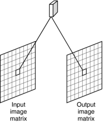
FIGURE 3-16 In a point operation, the value of the input image pixel is mapped onto the corresponding output image pixel.
The most commonly used point processing technique is called gray-level mapping. This is also referred to as “contrast enhancement,” “contrast stretching,” “histogram modification,” “histogram stretching,” or “windowing.” Gray-level mapping uses a look-up table (LUT), which plots the output and input gray levels against each other (Fig. 3-17).
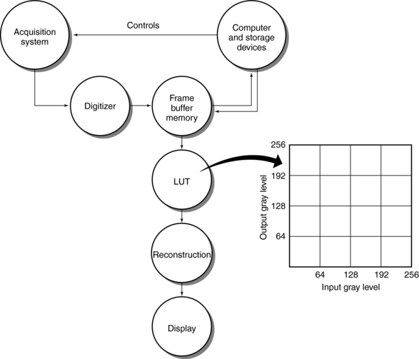
LUTs can be implemented with hardware or software for gray-level transformation. Figure 3-18 illustrates the transformation process. Gray-level mapping changes the brightness of the image and results in the enhancement of the display image.
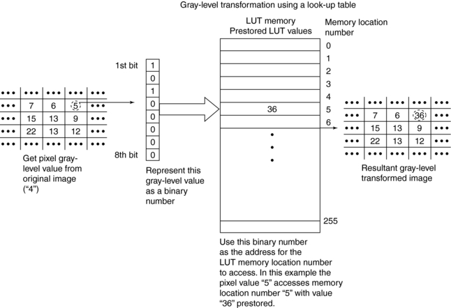
FIGURE 3-18 Gray-level transformation of an input image pixel. The algorithm uses the LUT to change the value of the input pixel (5) to 36, the new value of the output pixel. From Huang HK: PACS and imaging informatics: basic principles and applications, Hoboken, NJ, 2004, John Wiley.
Gray-level mapping results in a modification of the histogram of the pixel values. A histogram is a graph of the pixels in all or part of the image, plotted as a function of the gray level. A histogram can be created as follows:
1. Observe the image matrix (Fig. 3-19) and create a table of the number of pixels with a specific intensity value, as shown.
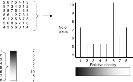
FIGURE 3-19 The creation of a histogram. A histogram is a graph of the number of pixels in the entire image or part of the image having the same gray levels (density values), plotted as a function of the gray levels. From Seeram E: Digital image processing, Radiol Technol 75:435-455, 2004. Reproduced by permission of the American Society of Radiologic Technologists.
2. Plot a graph of the number of pixels versus the gray levels (intensity or density values).
Histograms indicate the overall brightness and contrast of an image. If the histogram is modified or changed, the brightness and contrast of the image can be altered, a technique referred to as histogram modification, or histogram stretching. This is also an example of a point operation in digital image processing. If the histogram is wide, the resulting image has high contrast. If the histogram is narrow, the resulting image has low contrast. On the other hand, if the histogram values are closer to the lower end of the range of values, the image appears dark, as opposed to a bright image, in which the values are weighted toward the higher end of the range of values.
Local Operations
A local operation is an image processing operation in which the output image pixel value is determined from a small area of pixels around the corresponding input pixel (Fig. 3-20). These operations are also referred to as area processes or group processes because a group of pixels is used in the transformation calculation.
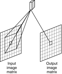
FIGURE 3-20 In the local operation, the value is determined from a small area of pixels surrounding the corresponding input pixel.
Spatial frequency filtering is an example of a local operation that concerns brightness information in an image. If the brightness of an image changes rapidly with distance in the horizontal or vertical direction, the image is said to have high spatial frequency. (An image with smaller pixels has higher frequency information than an image with larger pixels.) When the brightness changes slowly or at a constant rate, the image is said to have low spatial frequency. Spatial frequency filtering can alter images in several ways such as image sharpening, image smoothing, image blurring, noise reduction, and feature extraction (edge enhancement and detection).
There are two places to perform spatial frequency filtering: (1) in the frequency domain, which considers the FT, or (2) in the spatial domain, which uses the pixel values (gray levels) themselves.
Spatial Location Filtering: Convolution: Convolution, a general-purpose algorithm, is a technique of filtering in the space domain as illustrated in Figure 3-21.
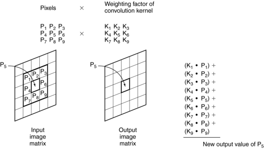
FIGURE 3-21 In convolution, the value of the output pixel is calculated by multiplying each input pixel by its corresponding weighting factor of the convolution kernel (usually a 3 × 3 matrix). These products are then summed.
The value of the output pixel depends on a group of pixels in the input image that surround the input pixel of interest: in this case, pixel P5. The new value for P5 in the output image is calculated by obtaining its weighted average and that of its surrounding pixels. The average is computed by using a group of pixels called a convolution kernel, in which each pixel in the kernel is a weighting factor, or convolution coefficient. In general, the size of the kernel is a 3 × 3 matrix. Depending on the type of processing, different types of convolution kernels can be used, in which case the weighting factors are different.
During convolution, the convolution kernel moves across the image, pixel by pixel. Each pixel in the input image, its surrounding neighbors, and the kernels are used to compute the value of the corresponding output pixel—that is, each pixel is multiplied by its respective weighting factor and then summed. The resulting number is the value of the center output pixel. This process is applied to all pixels in the input image; each calculation requires nine multiplications and nine additions. This can be time consuming, but special hardware can speed up this process.
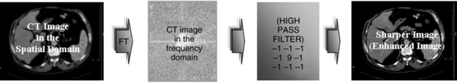
Spatial Frequency Filtering: High Pass Filtering: The high pass filtering process, also known as edge enhancement or sharpness, is intended to sharpen an input image in the spatial domain that appears blurred. The algorithm is such that first the spatial location image is converted into spatial frequencies by using the FT, followed by the use of a high pass filter that suppresses the low spatial frequencies to produce a sharper output image. This process is shown in Figure 3-22. The high pass filter kernel is also shown.
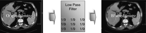
Spatial Frequency Filtering: Low Pass Filtering: A low pass filtering process makes use of a low pass filter to operate on the input image with the goal of smoothing. The output image will appear blurred. Smoothing is intended to reduce noise and the displayed brightness levels of pixels; however, image detail is compromised. This is illustrated in Figure 3-23. The low pass filter kernel is also shown.
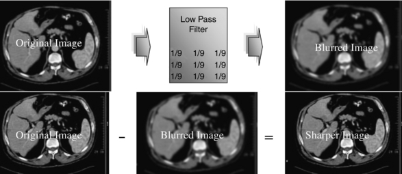
Spatial Frequency Processing: Unsharp (Blurred) Masking: The digital image processing technique of unsharp (blurred) masking uses the blurred image produced from the low pass filtering process and subtracts it from the original image to produce a sharp image, as illustrated in Figure 3-24. It can be see that the output image appears sharper.
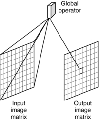
Global Operations
In global operations, the entire input image is used to compute the value of the pixel in the output image (Fig. 3-25). A common global operation is Fourier domain processing, or the FT, which uses filtering in the frequency domain rather than the space domain (Baxes, 1994). Fourier domain image processing techniques can provide edge enhancement, image sharpening, and image restoration.
Geometric Operations
Geometric operations are intended to modify the spatial position or orientation of the pixels in an image. These algorithms change the position rather than the intensity of the pixels, which is also a characteristic of point, local, and global operations. Geometric operations can result in the scaling and sizing of images and image rotation and translation (Castleman, 1996).
IMAGE COMPRESSION OVERVIEW
The evolving nature of digital image acquisition, processing, display, storage, and communications in diagnostic radiology has resulted in an exponential increase in digital image files. For example, the number of images generated in a multislice CT examination can range from 40 to 3000. If the image size is 512 × 512 × 12, then one examination can generate 20 megabytes (MB) of data, and up. A CT examination consisting of two images per examination with an image size of 2048 × 2048 × 12 will result in 16 MB of data. A digital mammography examination can now generate 160 MB of data. Additionally, Huang (2004) points out that “the number of digital medical images captured per year in the US alone is over pentabytes that is, 1015, and is increasing rapidly every year.” In this regard, it can safely be assumed that perhaps similar trends apply to Canada.
With the above in mind, image compression can solve the problems of image data storage and improve communication speed requirements for huge amounts of digital data (Seeram, 2004; Seeram and Seeram, 2008).
What Is Image Compression?
The literature is replete with definitions of image compression; however, one that stands out in terms of clarity is offered by Alan Rowberg, MD, of the Department of Radiology, University of Washington: “Digital compression refers to using one or more of many software and/or hardware techniques to reduce information by removing unnecessary data. The remaining information is then encoded and either transmitted or stored in an archive or storage media, such as tape or disk. In a process called decompression, the user’s equipment later decodes the information and fills in a representation of the data that was removed during compression.”
The above definition will serve as the basis for understanding what is meant by image compression.
Types of Image Compression
As mentioned earlier in this chapter, there are two types of image data compression; lossless or reversible compression, and lossy or irreversible compression. In the former, no information is lost when the image is decompressed or reconstructed; in the latter, there is some loss of information, when the image is decompressed (see Fig. 3-15).
Although it is not within the scope of this section to describe the technical details of the steps involved in image compression, the following points are noteworthy:
• In lossless or reversible compression, there is no loss of information in the compressed image data. Furthermore, lossless compression does not involve the process of quantization but makes use of image transformation and encoding to provide a compressed image.
• Lossy or irreversible compression involves at least three steps: image transformation, quantization, and encoding. As noted by Erickson (2002),
Transformation is a lossless step in which the image is transformed from gray scale values in the spatial domain to coefficients in some other domain. One familiar transformation is the Fourier Transform used in reconstruction Magnetic Resonance Images (MRI). Other transforms such as the Discrete Cosine Transform (DCT) and the Discrete Wavelet Transform (DWT) are commonly used for image compression. No loss of information occurs in the transformation step. Quantization is the step in which the data integrity is lost. It attempts to minimize information loss by preferentially preserving the most important coefficients where less important coefficients are roughly approximated, often as zero. Quantization may be as simple as converting floating point values to integer values. Finally, these quantized coefficients are compactly represented for efficient storage or transmission of the image.
There are a number of other issues relating to the use of irreversible compression in digital radiology, including the visual impact of compression (lossy compression) on diagnostic digital images and methods used to evaluate the effects of compression (Seeram, 2006). It is also well established that the quality of digital images plays an important role in helping the radiologist to provide an accurate diagnosis. At low compression ratios (8:1 or less), the loss of image quality is such that the image is still “visually acceptable” (Huang, 2004). The obvious concern that now comes to mind is related to what Erickson (2002) refers to as “compression tolerance,” a term he defines as “the maximum compression in which the decompressed image is acceptable for interpretation and aesthetics.”
Because lossy compression methods provide high to very high compression ratios compared with lossless methods, and keeping the term “compression tolerance” in mind, Huang (2004) points out that “currently lossy algorithms are not used by radiologists in primary diagnosis, because physicians and radiologists are concerned with the legal consequences of an incorrect diagnosis based on a lossy compressed image.”
Visual Impact of Irreversible Compression on Digital Images
The goal of both lossless and lossy compression techniques is to reduce the size of the compressed image, to reduce storage requirements, and to increase image transmission speed.
The size of the compressed image is influenced by the compression ratio (see definition of terms), with lossless compression methods yielding ratios of 2:1 to 3:1 (Huang, 2004), and lossy or irreversible compression having ratios ranging from 10:1 to 50:1 or more (Huang, 2004). It is well known that as the compression ratio increases, less storage space is required and faster transmission speeds are possible but at the expense of image quality degradation.
A recent survey of the opinions of expert radiologists in the United States and Canada (Seeram, 2006), on the use of irreversible compression in clinical practice showed that the opinions are wide and varied. This indicates that there is no consensus of opinion on the use of irreversible compression in primary diagnosis. Opinions are generally positive on the notion of image storage and image transmission advantages of image compression. Finally, almost all radiologists are concerned with the litigation potential of an incorrect diagnosis that is based on irreversible compressed images.
In providing a rationale for examining the trade-offs between image quality and compression ratio, an interesting experiment is suggested by Huang (2004) using five compressed CT images (512 × 512 × 12) with compression ratios of 4:1, 8:1, 17:1, 26:1, and 37:1 together with the original image. Next, determine the order of quality of the images, and finally, determine which compression ratio provides an image quality that can be used to provide a diagnosis. In the generalized results of this simple experiment, Huang states that “reconstructed images with compression ratios less than or equal to 8:1 do not exhibit visible deterioration in image quality. In other words, a compression ratio of 8:1 or less is visually acceptable. But visually unacceptable does not necessarily mean that the ratio is not suitable for diagnosis because this depends on what diseases are under consideration.”
IMAGE SYNTHESIS OVERVIEW
One of the advantages of digital image processing is image synthesis, and examples of image synthesis are the image reconstruction methods used in CT and MRI, and 3D imaging operations. Although image reconstruction is based on mathematical procedures, 3D techniques are based on computer graphics technology. Both CT image reconstruction and 3D imaging will be described in detail in later chapters, and therefore only highlights will be mentioned here.
Magnetic Resonance Imaging
The major system processes of MRI signal acquisition to image display are shown in Figure 3-26. First, magnetic resonance signals are acquired from the patient, who is placed in the magnet during the imaging procedure. These signals are high and low frequencies collected from the patient. The signals are subsequently digitized and stored in what is referred to as “k” space, which is a frequency domain space. Once k space is filled, the FT algorithm uses the data in k space to reconstruct magnetic resonance images, which are displayed on the monitor for viewing by a radiologist or technologist.
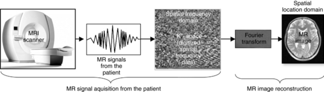
FIGURE 3-26 The major processes of MRI signal acquisition to image display. First, magnetic resonance (MR) signals are acquired from the patient, who is placed in the magnet during the imaging procedure. These signals are high and low frequencies collected from the patient. The signals are subsequently digitized and stored in what is referred to as “k” space, a frequency domain space. Image courtesy Philips Medical Systems.
Once displayed, images can be manipulated with special digital image processing software to perform such processing as windowing, and 3D image visualization, for example.
CT Imaging
A conceptual overview of CT imaging is shown in Figure 3-27. Attenuation data are collected from the patient by the detectors that send their electronic signals to the computer, having been digitized by the ADC. The computer then uses a special image reconstruction algorithm, referred to as the filtered back projection algorithm, to build up a digital CT image. This image must be converted to a gray scale image to be displayed on a monitor for viewing by the radiologist and the technologist.
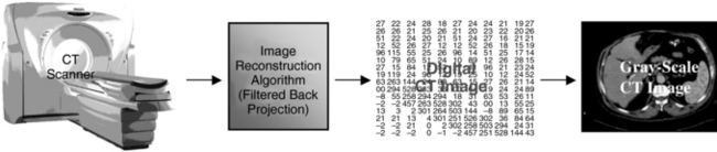
FIGURE 3-27 A conceptual overview of CT imaging. Image reconstruction is performed by the filtered back projection. See text for further explanation.
Displayed CT images can be manipulated with digital image processing software to perform such processing as windowing, image reformatting, and 3D image visualization.
Three-Dimensional Imaging in Radiology
3D imaging is gaining widespread attention in radiology (Beigelman-Aubry et al, 2005; Dalrymple et al, 2005; Neuman and Meyers, 2005; Seeram, 2004; Shekhar et al, 2003). Already 3D imaging is used in CT, MRI, and other imaging modalities with the goal of providing both qualitative and quantitative information from images to facilitate and enhance diagnosis.
The general framework for 3D imaging is shown in Figure 3-28. Four major steps are shown: data acquisition, creation of what is referred to as 3D space (all voxel information is stored in the computer), processing for 3D image display, and finally, 3D image display. Digital processing can allow the observer to view all aspects of 3D space, a technique referred to as 3D visualization. The application of 3D visualization techniques in radiology is referred to as 3D medical imaging.
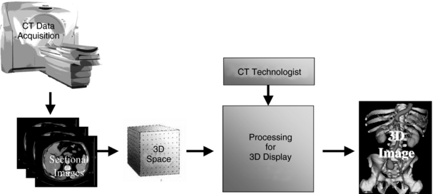
FIGURE 3-28 The general framework for 3D imaging. Four major steps are shown: data acquisition, creation of what is referred to as 3D space, processing for 3D image display, and finally 3D image display. Digital processing can allow the observer to view all aspects of 3D space, a technique referred to as 3D visualization. Image courtesy Philips Medical Systems.
Dr. Jayaram from the Department of Radiology at the University of Pennsylvania, an expert in 3D imaging, notes that there are four classes of 3D imaging operations: preprocessing, visualization, manipulation, and analysis. Because the visualization operations are now quite popular in digital imaging departments using CT and MRI scanners, it is noteworthy to highlight the major ideas of at least two 3D visualization techniques, surface rendering and volume rendering. Rendering is the final step in 3D image production. It is a computer program used to transform 3D space into simulated 3D images to be displayed on a two-dimensional computer screen.
Two classes of rendering techniques are used in radiology: surface rendering and volume rendering. Surface rendering is a simple procedure in which the surface of an object is created using contour data and shading the pixels to provide the illusion of depth. It uses only 10% of the data in 3D space and does not require a great deal of computation. Volume rendering, on the other hand, is a much more sophisticated technique. Volume rendering uses all the data in 3D space to provide additional information by allowing the observer to view more details inside the object, as is clearly illustrated in Figure 3-28. It also requires more computational power.
Applications of these rendering techniques are in several areas, including imaging the craniomaxillofacial complex, musculoskeletal system, the central nervous system, and cardiovascular, pulmonary, gastrointestinal, and genitourinary systems. 3D imaging is now popular in CT angiography (Fishman et al, 2006) and magnetic resonance angiography.
3D medical imaging uses stand-alone workstations featuring very powerful computers capable of a wide range of processing functions, including virtual reality imaging (VRI).
Virtual Reality Imaging in Radiology
VRI requires sophisticated digital image processing methods to facilitate the perception of 3D anatomy from a set of two-dimensional images (Huang, 2004; Kalender, 2005; Seeram, 2004). The vast amount of data collected by multislice CT scanners, for example, provides the opportunity to develop VRI imaging applications in radiology.
Virtual reality is a branch of computer science that immerses the users in a computer-generated environment and allows them to interact with 3D scenes. One common method that uses virtual reality concepts is virtual endoscopy. Virtual endoscopy is used to create inner views of tubular structures.
Virtual endoscopy involves a set of systematic procedures to be followed. These include data acquisition (careful selection of scan parameters in collecting data from the patient), image preprocessing (to optimize images before they are processed), 3D rendering, using both surface and volume rendering, and finally, image display, and analysis. Two examples of software tools available for interactive image assessment, include Philip’s Voyager and General Electric’s 3D Navigator (advanced visualization packages to allow the user to perform real-time navigation of structures using a “fly through” within and around tubular anatomy in the same manner a real endoscope is used. 3D imaging and VRI will be described in detail in a later chapter.
IMAGE PROCESSING HARDWARE
A basic image processing system consists of several interconnected components (Fig. 3-29). The major components are the ADC, image storage, image display, image processor, host computer, and DAC.
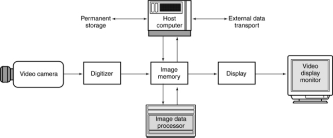
• Data acquisition: In Figure 3-29, the video camera is the data acquisition device. In CT this would be represented by the x-ray tube and detectors and the detector electronics.
• Digitizer: As can be seen in Figure 3-29, the analog signal is converted into digital form by the digitizer, or ADC.
• Image memory: The digitized image is held in storage for further processing. Several components are connected to the image store and provide input and output. The size of this memory depends on the image. For example, a 512 × 512 × 8 bit image requires a memory of 2,097,152 bits.
• DAC: The digital image held in the memory can be displayed on a television monitor. However, because monitors work with analog signals, it is necessary to convert the digital data to analog signals with a DAC.
• Internal image processor: This processor is responsible for high-speed processing of the input digital data.
• Host computer: In digital image processing, the host computer is a primary component capable of performing several functions. For example, the host computer can read and write the data in the image store and provide for archival storage on tape and disk storage systems. The host computer plays a significant role in applications that involve the transmission of images to another location, such as medical imaging.
CT AS A DIGITAL IMAGE PROCESSING SYSTEM
A number of imaging modalities in radiology use image processing techniques, including digital radiography and fluoroscopy, nuclear medicine, MRI, ultrasonography, and CT. The future of digital imaging is promising in that a wide variety of applications have received increasing attention, such as 3D imaging (Seeram and Seeram, 2008). The major image-processing operations in medical imaging that are now common in the radiology department are presented in Table 3-2.
TABLE 3-2
Common Digital Image Processing Operations Used in Diagnostic Digital Imaging Technologies
| Digital Imaging Modality | Common Image Processing Operations |
| CT | Image reformatting, windowing, region of interest, magnification, surface and volume rendering, profile, histogram, collage, image synthesis |
| MRI | Windowing, region of interest, magnification, surface and volume rendering, profile, histogram, collage, image synthesis |
| Digital subtraction angiography/digital fluoroscopy | Analytic processing, subtraction of images out of sequence, gray-scale processing, temporal frame averaging, edge enhancement, pixel shifting |
| Computed radiography/digital radiography | Partitioned pattern recognition, exposure field recognition, histogram analysis, normalization of raw image data, gray-scale processing (windowing), spatial filtering, dynamic range control, energy subtraction, etc. |
From Seeram E: Digital image processing, Radiol Technol 75:435-455, 2004. Reproduced by permission.
The basic components of a digital imaging system were illustrated in Figure 1-28. As a digital image processing system, CT fits into this scheme. In addition, similar steps in image digitization can be applied to the CT process, as follows:
1. First, divide the picture into pixels. In CT, the slice of the patient is divided into small regions called voxels (volume element) because the dimension of depth (slice thickness) is added to the pixel. The patient is scanned as the x-ray tube moves around the patient.
2. Next, sample the pixels. In CT, the voxels are sampled when x rays pass through them. This measurement is performed by detectors. The signal from the detector is in analog form and must be converted into digital form before it can be sent to the computer for processing.
3. The final step is quantization. In CT, the analog signal is also quantized and changed into a digital array for input into the computer. The digital data resulting from quantization are processed by the computer through a series of operations or techniques to modify the input image. In CT, the digital data are also subject to several processing algorithms so the output image can be displayed in a form suitable for human observation.
IMAGE PROCESSING: AN ESSENTIAL TOOL FOR CT
Image postprocessing and its associated techniques such as data visualization, computer-aided detection, and image data set navigation have recently been identified as major research areas in the transformation of medical Imaging (Andriole and Morin, 2006). Image postprocessing methods in CT are intended to enhance the diagnostic interpretation skills of the radiologist. Several examples of these methods include image reformatting to display axial images in the coronal, sagittal, and oblique views, maximum intensity and minimum intensity projections, curved reformatting, shaded surface display (SSD) and virtual reality, and physiologic imaging tools such as image fusion and CT perfusion. These methods will be described in detail in later chapters.
Digital image processing is now an essential tool in the CT and PACS environment, and already technologists and radiologists are actively involved in using the tools of image postprocessing, such as the digital image processing operations and techniques outlined in this chapter. Training programs for both technologists and radiologists are also beginning to incorporate digital image processing as part of their curriculum (Seeram and Seeram, 2008). A suggested list of topics for a course on image processing in CT would be the chapter outline at the beginning of this chapter. These topics can be expanded beyond the content of this chapter.
REFERENCES
Andriole, KP, Morin, R. Transforming medical imaging—the first SCAR TRIP Conference. J Digital Imaging. 2006;19:6–16.
Baxes, GA. Digital image processing: principles and applications. New York: John Wiley, 1994.
Beigelman-Aubry, D, et al. Multi-detector row CT and post-processing techniques in the assessment of lung diseases. Radiographics. 2005;25:1639–1652.
Castleman, KR. Digital image processing. Englewood Cliffs, NJ: Prentice Hall, 1996.
Dalrymple, NG, et al. Introduction to the language of three-dimensional imaging with multi-detector CT. Radiographics. 2005;25:1409–1428.
Erickson, BJ. Irreversible compression of medical images. J Digital Imaging. 2002;15:5–14.
Fishman, EK, et al. Volume rendering versus maximum intensity projection in CT angiography: what works best, when, and why. Radiographics. 2006;26:905–922.
Huang, HK. PACS and imaging informatics: basic prinicples and applications. Englewood Cliffs, NJ: John Wiley, 2004.
Kalender, WA. Computed tomography. Munich: Publicis MCD Werbeagentur Verlag, 2005.
Lindley, CA. Practical image processing in C. New York: John Wiley, 1991.
Luiten, AL. Digital: discrete perfection. Medicamundi. 1995;40:95–100.
Marion, A. Introduction to image processing. London: Chapman and Hall, 1991.
Neuman, J, Meyers, M. Volume intensity projection: a new post-processing techniques for evaluating CTA. Netherlands: Philips Medical Systems, 2005.
Pooley RA et al: Digital fluoroscopy, Radiographics 21:521-534, 2001.
Seeram, E. Computed tomography—physical principles, clinical applications and quality control. Philadelphia: WB Saunders, 2001.
Seeram, E. Digital image processing. Radiol Technol. 2004;75:435–455.
Seeram, E. Irreversible compression in digital radiology. Radiography. 2006;12:45–59.
Seeram E Using irreversible compression in digital radiology a preliminary study of the opinions of radiologists. Progress in Biomedical Optics and Imaging– Proceedings of the SPIE San DiegoCalifJuly 2006.
Seeram, E, Seeram, D. Image postprocessing in digital radiologya primer for technologists. Journal of Medical Imaging and Radiation Sciences. 2008;39:23–41.
Seibert, JA. Digital image processing: basics. In: Balter S, Shope TB, eds. A categorical course in physics: physical and technical aspects of angiography and interventional radiology. Oak Brook, Ill: Radiological Society of North America, 1995.