Chapter Twenty The interpretation of research evidence
Introduction
When researchers have demonstrated statistical significance within a study, what have they actually established? Statistical significance suggests that it is likely that there is a similar effect or phenomenon in the population from which the study sample has been drawn. However, it is not correct to assume that statistical significance necessarily implies clinical importance or usefulness. We must also establish the clinical or practical significance of our results following the step of demonstrating statistical significance.
Effect size
In a clinical intervention study, the effect size is the size of the effects that can be attributed to the intervention. The term effect size is also used more broadly in statistics to refer to the size of the phenomenon under study. For example, if we were studying gender effects on longevity, a measure of effect size could be the difference in mean longevity between males and females. In a correlational study, the effect size could be represented by the size of the correlation between the selected variables under study. There are many measures or indicators of effect size selected on the basis of the scaling of the outcome or dependent variable (Sackett et al 2000).
The concept of effect size can be illustrated by results from two student research projects supervised by the authors.
Study 1: Test–retest reliability of a force measurement machine
In the first study, the student was concerned with demonstrating the test–retest reliability of a device designed to measure maximum voluntary forces being produced by patients’ leg muscles under two conditions (flexion and extension). Twenty one patients took part and the reliability of the measurement process was tested by calculating the Pearson correlation between the readings obtained from the machine in question during two trials separated by an hour for each patient. The results are shown in Table 20.1. Both results reach the 0.01 level of significance.
Table 20.1 Pearson correlations between trials 1 and 2
| Flexion | Extension |
|---|---|
| 0.56 | 0.54 |
The student was ecstatic when the computer data analysis program informed that the correlations were statistically significant at the 0.01 level (indicating that there was less than a 1 in 100 chance that the correlations were illusory or actually zero). We were somewhat less ecstatic because, in fact, the results indicated that approximately 69% (1 − 0.562) and 71% (1 − 0.542) of the variation was not shared between the measurements of the first and second trial. In other words, the measures were ‘all over the place’, despite statistical significance being reached. Thus, far from being an endorsement of the measurement process, these results were somewhat of a condemnation. This is a classic example of the need for careful interpretation of effect size in conjunction with statistical significance.
Study 2: A comparative study of improvement in two treatment groups
The second project was a comparative study of two groups: one group suffering from suspected repetition strain injuries (RSI) induced by computer keyboard input and a group of ‘normals’. An Activities of Daily Living (ADL) assessment scale was used and yielded a ‘disability’ index of between 0 and 50. There were 60 people in each group. The results are shown in Table 20.2.
Table 20.2 Mean ADL disability scores
| RSI group | Normals | |
|---|---|---|
| Mean | 33.2 | 30.4 |
| Standard deviation | 1.6 | 1.2 |
The appropriate statistic for analysing these data happens to be the independent groups t test, although this is not important for understanding this example. The t value for these data was significant at the 0.05 level. Does this finding indicate that the difference is clinically meaningful or significant? There are two steps in interpreting the clinical significance of the results.
First, we calculate the effect size. For interval or ratio-scaled data the effect size ‘d’ is defined as:
where μ1 – μ2 refers to the difference between the population means and σ, the population standard deviation.
Since we rarely have access to population data we use sample statistics for estimating population differences. The formula becomes:
where  1 – 2 indicates the difference between the sample means and s1 refers to the standard deviation of the ‘normal’ or ‘control’ group. Therefore, for the above example, substituting into the equation yields:
In other words, the average ADL score of the people with suspected RSI was 2.33 standard deviations under the mean of the distribution of ‘normal’ scores. The meaning of d can be interpreted by using z scores. The greater the value of d, the larger the effect size.
Second, we need to consider the clinical implications of the evidence. It might be that the difference of 2.8 units of ADL scores is important and clinically meaningful. However, if one inspects the means, the differences are slight, notwithstanding the statistical significance of the results. This example further illustrates the problems of interpretation that may arise from focusing on the level of statistical significance and not on the effect sizes shown by the data.
When we say that the findings are clinically significant we mean that the effect is sufficiently large to influence clinical practices. It is the health workers rather than statisticians who need to set the standards for each health and illness determinant or treatment outcome. After all, even relatively small changes can be of enormous value in the prevention and treatment of illnesses. There are many statistics currently in use for determining effect size. The selection, calculation and interpretation of various measures of effect are beyond our introductory book, but interested readers can refer to Sackett et al (2000).
How to interpret null (non-significant) results
As we discussed in previous chapters, the researcher will sometimes analyse data that show no relationships or differences according to the chosen statistical test and criteria. In other words, the researcher cannot reject the null hypothesis. There are several reasons why the researcher may obtain a null result.
Therefore, if the researcher obtains a null result, one or more of the above explanations may be appropriate. There are, however, steps that can be taken to minimize the chance of missing real effects. In order to understand these measures, it is necessary again to invoke the table illustrating the possible outcomes of a statistical decision (as shown in Table 20.3).
Table 20.3 Statistical decision outcomes
| Reality | Decision: effect | Decision: no effect |
|---|---|---|
| Effect | Correct | ‘Miss’ Type II error |
| No effect | ‘False alarm’ Type I error | Correct |
There are four possible outcomes. On the basis of the statistical evidence you may: (i) correctly conclude there is an effect when there is indeed an effect; (ii) decide that there is an effect when there is not (this is a false alarm or Type I error); (iii) decide that there is not an effect when there really is (this is a miss or Type II error); or (iv) correctly decide there is not an effect when indeed there is not. The probability that researchers derive from their statistical tables is in fact the probability of making a false alarm or Type I error. This value does not tell us, however, how many times we will fail to identify a real effect. The probability of missing a real effect (or making a Type II error) is affected by the size of the actual effect and the number of cases included in our study. If you have large effects and large samples, the number of misses will be small. To detect a small effect size larger samples are needed.
Statistical power analysis
In statistical analysis we need to know how likely a miss is to occur. We can do this by calculating the statistical power of a design. The statistical power for a given effect size is defined as 1 – probability of a miss (Type II error or β). Thus, if the power of a particular analysis is 0.95, for a given effect size we will correctly detect the existence of the effect 95 times out of 100. Power is an important concept in the interpretation of null results. For example, if a researcher compared the improvements of two groups of only five patients under different treatment circumstances, the power of the analysis would almost certainly be low, say 0.1. Thus 9 times out of 10, even with an effect really present, the researcher would be unable to detect it.
It is essential to be careful in the interpretation of null results where they are used to demonstrate a lack of superiority of one treatment method over another, especially when there is a low number of cases. This may be purely a function of low statistical power rather than the equivalence of the two treatments. Unfortunately the calculation of statistical power is complicated and beyond the scope of this text. However, there are technical texts, such as Cohen (1988), that are available to look up the power of various analyses. There are also statistical programs that perform the same function. The best defence against low statistical power is a good-sized sample. Before quantitative research projects are approved by funding bodies or ethics committees, there is the requirement that sufficient data will be collected to identify real effects.
Effect size is a key determinant of both statistical and clinical significance. We are more likely to detect a significant pattern or trend in our sample data when a factor has a strong influence on health or illness outcomes. A very powerful treatment such as the use of antibiotics for bacterial infections could be demonstrated even in a small sample. Table 20.4 shows the association between effect size and sample size for determining statistical and clinical significance for the results of research and evaluation projects. The most useful results for clear decision making occur when both effect size and sample size are large. Where the effect size is large but the results are not statistically significant, it might be useful to replicate the study with a larger sample size. Unfortunately, in real research it might be difficult to obtain a large sample and the effect size, we discover, might be disappointingly small. It is for this reason that researchers make the best use of previous research and, if possible, complete pilot studies. The evidence from previous research and the results of pilot studies enable us to conduct power analyses for estimating the minimum sample size for detecting an effect if it is really there.
Table 20.4 The relationship between effect size, sample size and decision making
| Effect size | Sample size | |
|---|---|---|
| Large | Small | |
| High | Both statistical and clinical significance are likely to be demonstrated | Statistical significance might not be demonstrated, but clinical significance would be indicated |
| Low | Statistical significance would be likely, but the results might not indicate clinically applicable outcomes | Neither statistical nor clinical significance is likely. Statistically significant results might result in Type I error |
Table 20.5 shows how evidence for statistical and clinical significance can be combined to interpret the findings of a study. A clear positive outcome is when there is strong evidence for both clinical and statistical significance. In this case we are confident that the information obtained is clinically useful and generalizable to the population. Another clear finding, provided that the sample size was adequate, is the lack of clear treatment effect. Such negative findings can be very useful in eliminating false hypotheses or ineffectual treatments.
Table 20.5 How to interpret findings
| Clinical significance | Statistical significance | |
|---|---|---|
| Yes | No | |
| Yes | Clear: strong evidence for treatment effect | Inconclusive: need for further research (e.g. with larger samples) |
| No | Inconclusive: suggests findings might not be meaningful – need further research | Clear: strong evidence for lack of a treatment effect |
Acknowledgement: We are grateful to Dr. Paul O’Halloran (La Trobe University) for this table.
Clinical decision making
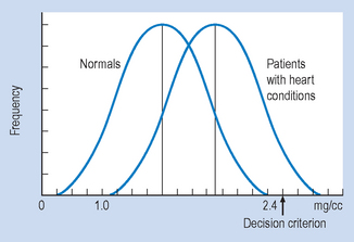
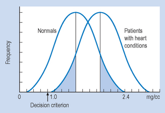
The decisions confronting a clinician making a diagnosis on the basis of uncertain information are similar to the scientist’s hypothesis testing procedure. As a hypothetical example, assume that a clinician wishes to decide whether a patient has heart disease on the basis of the cholesterol concentration in a sample of the patient’s blood. Previous research of patients with heart disease and ‘normals’ has shown that, indeed, heart patients tend to have a higher level of cholesterol than normals.
When the frequency distributions of cholesterol concentrations of a large group of heart patients and a group of normals are graphed, they appear as shown in Figure 20.1. You will note that, if patients present with a cholesterol concentration between 1.0 and 2.4 mg/cc, it is not possible to determine with complete certainty whether they are normal or have heart disease, due to the overlap of the normal and heart disease groups in the cholesterol distribution.
Therefore, the clinician, like the scientist, has to make a decision under uncertainty: to diagnose pathology (that is, reject the null hypothesis) or normality (that is, retain the null hypothesis). The clinician risks the same errors as the scientist, as shown in Table 20.6.
Table 20.6 Clinical decision outcomes
| Reality | Decision: pathology | Decision: no pathology |
|---|---|---|
| No pathology | ‘False alarm’ Type I error | Correct decision |
| Pathology | Correct decision | ‘Miss’ Type II error |
The relative frequency of the type of errors made by the clinician can be altered by moving the point above which the clinician will decide that pathology is indicated (that is, the decision criterion). For example, if clinicians did not bother their colleagues or patients with false alarms (Type I errors), they might shift the decision criterion to 2.5 mg/cc (Fig. 20.1). Any patient presenting with a cholesterol level below 2.5 mg/cc would be considered normal. In this particular case, with a decision point of 2.5 mg/cc, no ‘false alarms’ would occur. However, a huge number of people with real pathology would be missed (Type II errors).
If clinicians value the sanctity of human life (and their bank balance after a successful malpractice suit) they will probably adjust the decision criterion to the point shown in Figure 20.2. In this case, there would be no misses but lots of false alarms.
Thus, most clinicians are rewarded for adopting a conservative decision rule, where misses are minimized, by receiving lots of false alarms. Unfortunately, this generates a lot of useless, expensive and sometimes even dangerous clinical interventions.
Summary
In the interpretation of a statistical test, the researcher calculates the statistical value and then compares this value against the appropriate table to determine the probability level. If the probability is below a certain value (0.05 is a commonly chosen value), the researcher has established the statistical significance of the analysis in question. The researcher must then interpret the implications of the results by determining the actual size of the effects observed. If these are small, the results may be statistically significant but clinically unimportant. Statistical significance does not imply clinical importance.
A null result (indicating no effects) must be carefully interpreted. It is possible that the researcher has missed an effect because of its small size and/or insufficient cases in the analysis. The statistical analysis measures the chance of correctly detecting a real effect of a given size. Thus, a null result may be a function of low statistical power, rather than there being no real effect. It is necessary to carry out a statistical power analysis before undertaking a research project.
There are several criteria, beyond statistical significance, which need to be considered before making decisions concerning the clinical relevance of investigations. The most important criterion is a large and consistent effect size. In addition to effect size, the determination of clinical significance is influenced by values and economic limitations concerning the administration of health care in a given community.
Self-assessment
Explain the meaning of the following terms: