Introduction to: Discussion, questions and answers
Inferential statistical tests arise from the desire of clinical researchers to generalize from the data they have collected in a sample to the population from which the sample has been drawn. ‘Is what I have found in my sample a true representation of the population (and hence other samples)?’ is the basic question to be answered through the use of inferential statistical tests.
Inferential statistical tests all have the same basic format. The data are processed using the appropriate calculation procedure (often with the support of a computer program) and the value of the statistic is calculated. This value obtained is then compared with a table of known values in order to interpret the outcome of the statistical test. This is very much like the application of clinical tests where, in order to interpret the value of the test result, it is compared with a known standard. As with the clinician, the clinical researcher needs to know which test to choose in which circumstance. It would not be appropriate to try to measure the weight of a patient by giving her an X-ray. Similarly, it is not appropriate to use a χ2 test when the t test is required. It is beyond the scope of an introductory text to have an extended discussion of the various types of statistical tests and when they might be used (although it should be noted that there are many fewer statistical than clinical tests). However, it is essential that the student understands the basic use of inferential tests.
Consider the following analysis using χ2. This statistic is designed to test the relationship between variables with nominal or categorical scales (i.e. the values are categories).
The clinical researcher is using the χ2 test to examine the relationship between length of stay in hospital and the rate of unplanned readmissions. These data are described more fully in Section 5. The goal is to determine whether there is a stat-istically significant association between the two variables. The raw data appear in Table D20.1.
Table D20.1 Average lengths of stay and readmission rates per 100 patients for patients with fractured neck of femur at 30 hospitals
| Hospital | Average length of stay (days) | Unplanned readmission rates per 100 patients |
|---|---|---|
| 1 | 11.100 | 7.800 |
| 2 | 11.200 | 6.500 |
| 3 | 11.200 | 4.300 |
| 4 | 11.200 | 5.500 |
| 5 | 11.700 | 5.100 |
| 6 | 12.100 | 5.200 |
| 7 | 12.100 | 5.000 |
| 8 | 12.100 | 4.900 |
| 9 | 12.300 | 4.800 |
| 10 | 12.400 | 3.400 |
| 11 | 12.400 | 5.000 |
| 12 | 12.500 | 4.300 |
| 13 | 13.100 | 3.900 |
| 14 | 13.100 | 3.300 |
| 15 | 13.200 | 4.700 |
| 16 | 13.200 | 4.500 |
| 17 | 13.200 | 5.500 |
| 18 | 13.300 | 4.100 |
| 19 | 13.700 | 3.200 |
| 20 | 13.900 | 3.400 |
| 21 | 14.100 | 3.500 |
| 22 | 14.200 | 3.400 |
| 23 | 14.200 | 6.000 |
| 24 | 14.900 | 4.400 |
| 25 | 15.300 | 3.300 |
| 26 | 15.400 | 4.200 |
| 27 | 15.400 | 4.300 |
| 28 | 15.500 | 4.100 |
| 29 | 16.300 | 3.200 |
| 30 | 22.400 | 3.300 |
As demonstrated in Section 5, we could use the Pearson correlation to analyse these data. However, to illustrate the use of χ2 we will recode the data to categorical data and use this technique. The data will be recoded using the averages for each variable to convert the data from ratio data to categorical data. For example, all those cases (hospitals) with a mean length of stay of 13.6 days or greater will be considered as having an ‘above-average’ length of stay. Those cases (hospitals) with a stay below 13.6 days will be considered as having a ‘below-average’ length of stay. The same procedure will be followed for readmission rates of 4.47 or greater. These are the respective means for the two variables shown in Table D20.1. The recoded data appear as Table D20.2.
Table D20.2 Recoded average lengths of stay and readmission rates per 100 patients for patients with fractured neck of femur at 30 hospitals
| Hospital | Average length of stay (days) | Unplanned readmission rates per 100 patients |
|---|---|---|
| 1 | Below average | Above average |
| 2 | Below average | Above average |
| 3 | Below average | Below average |
| 4 | Below average | Above average |
| 5 | Below average | Above average |
| 6 | Below average | Above average |
| 7 | Below average | Above average |
| 8 | Below average | Above average |
| 9 | Below average | Above average |
| 10 | Below average | Below average |
| 11 | Below average | Above average |
| 12 | Below average | Below average |
| 13 | Below average | Below average |
| 14 | Below average | Below average |
| 15 | Below average | Above average |
| 16 | Below average | Above average |
| 17 | Below average | Above average |
| 18 | Below average | Below average |
| 19 | Above average | Below average |
| 20 | Above average | Below average |
| 21 | Above average | Below average |
| 22 | Above average | Below average |
| 23 | Above average | Above average |
| 24 | Above average | Below average |
| 25 | Above average | Below average |
| 26 | Above average | Below average |
| 27 | Above average | Below average |
| 28 | Above average | Below average |
| 29 | Above average | Below average |
| 30 | Above average | Below average |
From these data we can construct a contingency table which shows the relationship between the two newly coded variables. We do this by counting the number of times the 30 cases fall into the appropriate categories.
As can be seen from Table D20.3, only one hospital with an above-average length of stay had an above-average readmission rate, while 11 hospitals with above-average lengths of stay had below-average readmission rates.
Table D20.3 Contingency table of relationship between average length of stay and readmission rates at 30 hospitals for patients with fractured neck of femur
| Unplanned readmission rate | ||
|---|---|---|
| Length of stay | Above average | Below average |
| Above average | 1 | 11 |
| Below average | 12 | 6 |
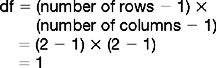
These data can be subjected to χ2 analysis. If these calculations are performed, we obtain a χ2 value of 9.98, df = 1, p < 0.01. In other words there is a statistically significant association between length of stay and readmission rates for the 30 hospitals. This confirms the analysis conducted in Section 5.