Chapter 39 Magnetic resonance imaging
Chapter contents
39.1 Aim
The aim of this chapter is to describe the technique of magnetic resonance imaging (MRI), which is a powerful imaging tool capable of providing both anatomical and functional information on living tissues. Some key adjustable MR imaging parameters, such as TR (time to repetition) and TE (time to echo), are introduced and the appearances of standard MR image sequences are presented in order to allow their recognition in clinical practice. Available scanner technologies and MRI safety issues are summarized.
39.2 Key principles of MRI
From the middle of the twentieth century, the technique of nuclear magnetic resonance (NMR) was widely used in laboratories to study the signatures and concentrations of chemicals. Bloch and Purcell, working independently, had noted in 1946 that chemical samples placed in a strong magnetic field, when subjected to radiofrequency (RF) radiations at specific resonant frequencies, returned detectable and characteristic radiofrequency signals. At this point it would be useful to explain why this occurs. Atomic nuclei (hence the term nuclear in NMR) have an angular momentum or spin, which means that they rotate on their axes, rather like tiny planets. They also have magnetic dipole moments. Note that a ‘moment’ in this context means a vector quantity with magnitude and direction, not a brief moment of time! In MRI, the term ‘spin’ is commonly used to refer to the rotating magnetic field orientation of an individual atomic nucleus, although strictly the term magnetic dipole moment is more correct.
Moving charges such as electrons produce a magnetic field and similarly a spinning positively charged proton can possess a magnetic field. It may seem surprising that spinning neutrons also possess magnetic fields. This is because they, like protons, are composed of smaller subatomic particles, some of which are charged. So we can think of both protons and neutrons contributing to the overall magnetic properties of atomic nuclei.
Normally the magnetic dipole moments of individual atomic nuclei, whether in a chemical sample or in a human body, are aligned randomly in all directions. There is no overall net magnetization. But if a powerful and uniform magnetic field is applied, the individual magnetic dipole moments tend to align:
• either with the external magnetic field (which is referred to in MRI as parallel or ‘spin-up’). This is a low-energy state.
• or against the external magnetic field (which is referred to in MRI as antiparallel or ‘spin-down’). This is a high-energy state.
There is normally a slight excess of magnetic dipole moments in the low-energy ‘spin down’ state, an excess which increases as the external magnetic field strength increases. These states are illustrated in Figure 39.1 (see page 288). The rotational or precessional frequency of the magnetic dipole moments is directly proportional to the external magnetic field strength. The Larmor equation describes this relationship:
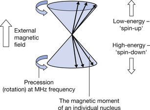
Figure 39.1 The precession of individual magnetic dipole moments placed in a strong external magnetic field.

where ω is the precessional frequency in Hertz, B0 is the magnetic flux density of the external magnetic field in tesla and γ is a constant known as the gyromagnetic ratio. This dependence of precessional frequency on local magnetic field strength (since γ is constant) is a very important principle in MRI and has a host of applications.
The gyromagnetic ratio is set according to which chemical element is being used in NMR or MRI. The gyromagnetic ratio of hydrogen-1 is 42.6 MHz (million cycles per second) per tesla. Thus, hydrogen-1 nuclei precess at 42.6 MHz at a magnetic flux density of 1 tesla. Hydrogen is very abundant in water and biological molecules like fats, proteins and carbohydrates. This, coupled with the fact that its most common (H-1) nucleus has a strong magnetic signal, enables us to visualize many body tissues effectively.
Table 39.1 lists the gyromagnetic ratios of some nuclei used in MRI and magnetic resonance spectroscopy (MRS). MRI provides images of human anatomy, while MRS is an adaptation of NMR used to measure the strength of chemical signatures in living tissues, by providing spectra. Only hydrogen-1 has sufficient abundance and signal in the body to provide images.
Table 39.1 Some atomic nuclei used in MRI and MRS
| NUCLEUS (MASS NUMBER) | GYROMAGNETIC RATIO (MHz PER TESLA) | RELATIVE SIGNAL STRENGTH | NOTES |
|---|---|---|---|
| Hydrogen-1 | 42.6 | 100 | |
| Carbon-13 | 10.7 | 1.45 | |
| Fluorine-19 | 40.1 | 83 | |
| Phosphorus-31 | 17.2 | 6.6 |
It can be seen in Table 39.1 that nuclei which return a useful signal in MRI and MRS all have an odd number of nucleons (odd mass numbers). This is not a coincidence. The magnetic moments of individual nucleons tend to ‘pair up’ and cancel each other out in nuclei with even mass numbers, leaving no net magnetization. This is rather analogous to a situation that occurs among electrons orbiting atomic nuclei – these electrons tend to pair up in ‘spin-up’ and ‘spin-down’ states in chemical bonds, while unpaired electrons are chemically reactive.
The frequency of the returning radio wave signals received from nuclei in chemical samples or living tissues is influenced by the local chemical environment. This is largely due to the presence of electrons in chemical bonds, which slightly ‘shield’ nuclei to varying extents from the external magnetic field. Thus hydrogen nuclei (for example) in different chemical molecules (such as water, lactate, fat) precess at very slightly different speeds, according to the Larmor equation. This creates frequency shifts, known as chemical shifts in the radio wave signals received within a spectrum. This effect is the basis of nuclear magnetic resonance and magnetic resonance spectroscopy. In MRI, the chemical shift effect can result in artefacts. Figure 39.2 shows a hydrogen-1 spectrum obtained in an MRS procedure.
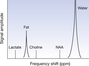
Figure 39.2 A hydrogen-1 (proton) spectrum obtained from MR spectroscopy. Note that, to avoid confusion, frequency is plotted from low (left) to high (right) on the x-axis, although in practice this would be plotted in reverse order. Units of frequency are typically parts per million (ppm) frequency shift. The shift between fat and water is 3.5 ppm. The peaks for water and fat are very large (larger than shown) relative to other chemicals. Lactate levels increase in anaerobic conditions, for example in tumours. Choline is a substrate for cell synthesis and reflects cell proliferation. NAA (N-acetyl aspartate) is a marker for neurons.
Magnetic resonance spectroscopy is a powerful tool for providing chemical information on lesions such as tumours, but requires large voxels, high magnetic field strength, a very homogeneous magnetic field and cannot provide 2D or 3D images of human anatomy.
A high magnetic field strength in the order of 1.5 tesla or greater is needed in MRS in order to increase the frequency shift (chemical shift) between chemicals so that they show up more clearly as distinct spectral peaks. For example, although the shift between water and fat is always 3.5 parts per million, the actual frequency difference is three times greater at a field strength of 3 tesla (where hydrogen-1 precessional frequency is 42.6×3=127.8 MHz) than at 1 tesla (where hydrogen-1 precessional frequency is 42.6 MHz).
In 1971, Raymond Damadian provided an impetus to the development of actual clinical imaging using strong magnetic fields (magnetic resonance imaging or MRI) by suggesting that the radio wave signal relaxation times of different tissues might be indicative of the degree of tumour malignancy. Paul Lauterbur provided the first 2D MR image of a chemical sample in 1973 and suggested the term zeugmatography for the technique. Developments in clinical MRI continued in the United States and in the United Kingdom, led by Peter Mansfield and colleagues in the latter, with the first clinical scanners appearing in about 1980.
Clinical MRI almost always uses hydrogen-1 nuclei as the ‘MR-active’ signal source in the human body. When radiofrequency (RF) radiations are applied to a patient’s body, placed in a powerful magnetic field, at precisely the Larmor or precessional frequency of the hydrogen nuclei, then resonance occurs and energy is transferred to the nuclei. Subsequently two types of tissue ‘relaxations’ or releases of radio energy from the patient (resulting in signals) occur simultaneously.
• The longitudinal relaxation process occurs relatively slowly over a time period typically up to several hundred milliseconds. In this process the overall tissue magnetization, which has been briefly ‘flipped’ by a flip angle α towards 90° from the external magnetic field direction by the RF energy input, subsequently returns to a position of 0°, parallel to the magnetic field. This is the basis of the T1 signal component in MRI.
• The transverse relaxation process occurs relatively quickly over a time period typically up to several tens of milliseconds. In this process the rotating magnetic moments of individual nuclei, which have been brought briefly into line (or in phase) by the RF energy input, subsequently fan out (or dephase). This is the basis of the T2 signal component in MRI.
These relaxation processes are illustrated in Figures 39.3 and 39.4 (see page 290).
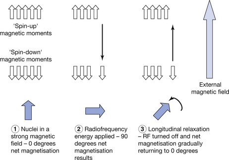
Figure 39.3 The longitudinal relaxation process for the magnetic moments of hydrogen nuclei in a strong magnetic field. Before RF energy is applied, there is a small excess of low-energy ‘spin-up’ magnetic moments, giving an overall magnetization of 0° (up in the diagram) parallel to the magnetic field. On the application of RF at the resonance frequency, some spins are promoted to the higher-energy ‘spin-down’ state and net magnetization is towards 90°. Removal of the RF energy causes gradual ‘recovery’ of overall net magnetization to 0°, with some spins returning to the low-energy state.
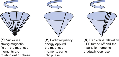
Figure 39.4 The transverse relaxation process for the magnetic moments of hydrogen nuclei in a strong magnetic field. Before RF energy is applied, the magnetic moments of individual nuclei are all precessing at the Larmor frequency and ‘out of step’ (out of phase) with each other. Think of them rotating at points occupying every minute of a clock face. When RF energy is applied, the magnetic moments all come briefly ‘into step’ (in phase), as if they were all rotating together in the 12 o’clock position on a clock face. When the RF energy is turned off, the magnetic moments all dephase.
The two processes of i) ‘flipping’ the overall magnetization towards 90° relative to the external magnetic field, and ii) putting the magnetic moments in phase, induces a strong electrical signal in a receiver coil placed at 90° to the main magnetic field. The frequency of this signal matches the precessional frequency of the magnetic moments of the nuclei. When they are all in phase, a powerful alternating current is induced in the receiver coil. For an analogy, we could think of the way a bright rotating lighthouse beam sweeps periodically towards an observer. Imagine if the light fanned out and went diffuse – the beam would be less effective. As the magnetic moments of the nuclei dephase in MRI, the signal in the receiver coil similarly fades out. This is called a free induction decay (FID).
The longitudinal relaxation process is also termed longitudinal recovery, or spin-lattice relaxation. It occurs relative to the longitudinal plane (0°) and involves transfer of energy to the atomic lattice of the material. Note that although RF energy causes heating of human tissues, this is via electromagnetic induction and not flipping of the magnetic moments of nuclei.
The transverse relaxation process is also called spin-spin relaxation, because the process of dephasing occurs within the transverse plane and occurs between magnetic moments (spins).
Some important practical features of the longitudinal and transverse recovery processes are summarized in Table 39.2 (see page 291).
Table 39.2 Relaxation of the radiofrequency signal in MRI
| LONGITUDINAL RELAXATION | TRANSVERSE RELAXATION |
|---|---|
| Occurs slowly overall | Occurs quickly overall |
| Fat relaxes relatively quickly and water slowly | Fat relaxes relatively quickly and water slowly |
| Is the basis of T1 weighted imaging | Is the basis of T2 weighted imaging |
| Using T1 image weighting, fat appears bright and water appears dark | Using T2 image weighting, fat appears grey and water appears bright |
| Good for depicting anatomy | Good for depicting pathology (fluid filled) |
| Tissues which enhance with gadolinium contrast agent appear bright with T1 weighting | Tissues which enhance with iron oxide contrast agent appear dark with T2 weighting |
39.3 Image weightings, sequences and appearances
Leaving the physics aside for a moment, it is very important to be able to interpret the appearance of MRI images. In this section, we will first consider the appearances of T1, T2, proton density and fat or fluid ‘saturated’ images.
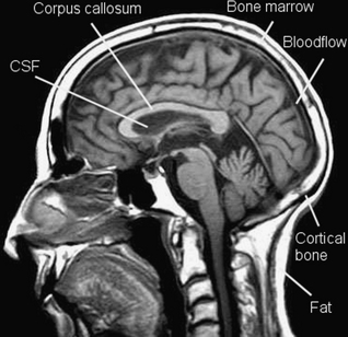
Remember that on a T1 weighted image, in terms of the longitudinal recovery process, fat relaxes quickly and appears bright. Fluid relaxes slowly and appears dark.
Look at Figure 39.5, a T1 weighted image. The subcutaneous fat appears bright. Cerebrospinal fluid in the lateral ventricle appears dark. White matter in the corpus callosum of the brain appears relatively bright, because it contains axons with fatty myelin sheaths. Cortical bone appears dark, because its hydrogen-1 atoms are tightly bound within a crystalline lattice and transverse relaxation between spins occurs so quickly that no signal can be sampled. But bone marrow appears bright, because it contains fat. Flowing blood in the sagittal venous sinus appears dark, because in spin echo imaging the flowing hydrogen atoms pass through an imaging slice before they can return a signal. This is known as the time of flight effect.
On an MRI image, you may see the terms TR (time to repetition) and TE (time to echo) stated. The TR is the time in milliseconds between one radio wave excitation of the atomic nuclei and the next. The TE is the time in milliseconds between a radio wave excitation and the received signal (which is called an echo). This is not to be confused with echoes in ultrasound! T1 weighted images use a short TR and short TE and this contributes to making a T1 image relatively quick to acquire. It is often relatively free from motion blur. Figure 39.6 (see page 292) illustrates the terms TR and TE.
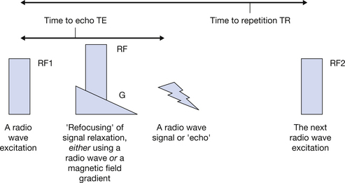
Figure 39.6 The TR is the time between two RF excitation pulses. The TE is the time between an RF excitation pulse and a signal. Adjustment of the TR and TE affects the image weighting in MRI.
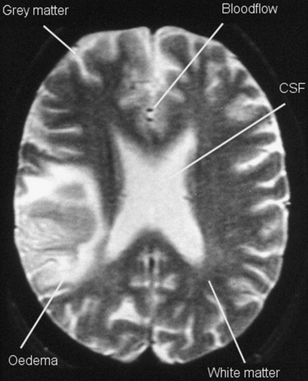
Now let’s look at Figure 39.7 (see page 292), a T2 weighted image. On a T2 weighted image, fluid appears bright. Fluid relaxes more slowly than fat in terms of the transverse recovery process. The bright signal from CSF in the lateral ventricles and oedema surrounding a brain tumour can be seen. Notice that fat and cortical bone appear grey or dark (the latter for the reason considered above) and are not well seen here. Grey matter, which contains many fluid-containing cell bodies, appears relatively bright, while the fatty myelinated axons of white matter appear grey. Once again flowing blood, seen here in two end-on blood vessels, does not give a signal as this is a spin echo image. T2 weighted images use a long TR and long TE and this contributes to making a T2 image relatively slow to acquire. It is more often affected by motion blur than a T1 image.
In MRI, a gradient is a linear and regular variation in magnetic flux density, from low to high. There are many uses of gradients in MRI. In gradient echo imaging, a magnetic field gradient is used to refocus a signal, giving a gradient echo. Gradient echo MRI sequences are fast and have the characteristic that flowing blood appears bright. (Spin echo sequences, which use an RF pulse to refocus the signal and give a spin echo are relatively slow, high contrast and give no signal from flowing blood.) Gradients are also used in MRI to obtain slices in the sagittal, coronal and axial planes. Changing a gradient in a regular way across a patient alters the local precessional frequencies and phases of the rotating magnetic moments of hydrogen-1 nuclei. This enables a unique ‘address’ of the nuclei to be obtained. Direct multiplanar imaging is a major strength of MRI.
You may also encounter proton density weighted images in MRI. Such images tend to appear rather low in contrast compared with T1 or T2 images and are simply based on the number of ‘protons’ (in fact the numbers of hydrogen-1 nuclei) present within the image. Tissues with a high ‘proton density’ such as fluid and fat appear relatively bright. To achieve a proton density image, the contribution of T1 and T2 weighting must be minimized and so a long TR (to reduce T1 weighting) and a short TE (to minimise T2 weighting) are used.
There are a number of imaging techniques commonly used in MRI, as summarized in Table 39.3.
Table 39.3 Common imaging techniques used in MRI
| TECHNIQUE | EXPLANATION |
|---|---|
| Spin echo (SE) | A standard MRI technique which uses a signal refocusing RF pulse to generate a spin echo |
| STIR (short time inversion recovery) | A spin echo sequence based on RF pulses which reduces fat signal and increases the conspicuity of fluid-containing pathologies |
| FLAIR (fluid attenuated inversion recovery) | A spin echo sequence based on RF pulses which reduces fluid signal and increases the conspicuity of pathologies which could otherwise be masked by fluid |
| Fat saturation or ‘fat sat’ | An alternative means of reducing fat signal which works by targeting RF pulses at the precessional frequency of fat |
| Inversion recovery (IR) | A spin echo sequence which enables contrast between different tissues to be amplified and finely controlled |
| Dual echo | A spin echo sequence which contains two refocusing RF pulses and simultaneously provides proton density and T2 image information |
| FSE (fast spin echo), also called TSE (turbo spin echo) | A rapid spin echo sequence which includes several signal-refocusing RF pulses rather than just one |
| RARE (rapid acquisition with relaxation enhancement) or single-shot FSE | A very fast spin echo sequence which uses a very long train of refocusing RF pulses and obtains all information from an imaging slice in a ‘single shot’ |
| Gradient echo (GE) | A standard and fast MRI technique which uses a signal refocusing gradient to generate a gradient echo. Results in T2 weighting in which magnetic susceptibility effects are strong |
| Flowing blood appears bright | |
| Echo planar imaging (EPI) | A very fast gradient echo sequence which uses a very long train of refocusing gradients and obtains all information from an imaging slice in a ‘single shot’ or ‘multi-shot’ |
| Magnetic resonance angiography (MRA) | A gradient echo technique in which flowing blood signal is amplified and stationary tissue signal is suppressed |
| Includes time of flight (TOF) and phase contrast (PC) techniques which do not use gadolinium contrast media and contrast enhanced (CE) techniques which do |
39.4 MRI equipment – scanners and coils
There are three main types of MRI magnet systems in clinical use, with most systems being superconducting, since these offer the greatest field strength and image quality. High-field magnets, which typically operate at magnetic flux densities of 1.5 to 3 tesla, offer the advantages of high signal-to-noise ratios (which permit good image resolution and image scanning) and suitability for a range of applications including MR spectroscopy, diffusion imaging and functional imaging.
• Superconducting magnets typically operate at magnetic flux densities up to 3 tesla for clinical use. They are powerful electromagnets whose coils of wire (typically niobium–tin or niobium–titanium alloy) show the phenomenon of zero electrical resistance at temperatures of around 4 Kelvin (−269°C) when cooled by liquid helium. The magnetic field is typically parallel to the floor, along the long axis of a patient, and is homogeneous over a wide volume. Signal-to-noise ratio is excellent. Drawbacks include large purchase and running costs, a large fringe magnetic field (which increases hazards and interference) and claustrophobia. Once ‘ramped-up’, such magnets cannot be switched off, except via a costly boil-off or ‘quench’ of liquid helium.
• Resistive magnets are powerful electromagnets which rely on a large current density to create a strong magnetic field and operate at room temperature. Combination with permanent magnet materials can permit magnetic flux densities up to about 1 tesla. Such magnets often have a magnetic field vertical to the floor and provide the advantages of reduced claustrophobia (being ‘open’ designs) and reduced fringe field (which reduces hazards). They can also be switched off. However they tend to suffer from poor field homogeneity and low signal-to-noise ratio.
• Permanent magnet designs are based around large ferromagnetic iron or alloy cores and may be quite bulky if even a moderate field strength is to be achieved. Relatively little used in clinical practice, they provide advantages of low fringe field and running costs but suffer from poor signal-to-noise ratio and field homogeneity.
Coils found in MRI are tuned to radio wave frequencies in the megahertz range employed. Transmit coils, as the name indicates, transmit RF waves into the patient at a finely controlled range of frequencies which affect slice thickness and image quality. They tend to be of ‘volume coil’ or bird cage designs which surround an area of patient anatomy. They may also have transmit–receive qualities. Receiver coils are designed to permit a good signal-to-noise ratio and should be positioned parallel to the external magnetic field and as close as possible to the anatomy of interest. Like transmit coils, they utilize Faraday’s laws of electromagnetic induction. Small coils tend to provide good signal-to-noise ratios but poor volume coverage. This can be addressed by phased arrays of individual coils. Whole-body imaging can be provided by extended arrays of coils.
39.5 MRI bioeffects and safety
Although MRI does not generate ionizing radiation and is not thought to induce cancers, there are a large number of biological effects of MRI scanning, some of which can be fatal. This is a surprise to many people. Thus MRI must be operated within strict guidelines, although most effects are transient and reversible. Sources of hazard in MRI arise from:
• the static (time-invarying) external magnetic field which operates at magnetic flux densities of several tesla
• varying magnetic fields applied by magnetic field gradients
• radiofrequency electromagnetic fields used to excite nuclear spins.
The projectile effect is the most dramatic demonstration of the influence of the static magnetic field. This exerts a rotational torque and translational force on ferromagnetic objects, tending to align them with the field and draw them towards greater magnetic flux densities. An exclusion zone of 5 gauss surrounds an MRI scanner, designed to prevent objects like scissors and oxygen cylinders from becoming projectiles and also to prevent damage to magnetically sensitive devices like pacemakers. The static field also affects the T-wave amplitude in the cardiac cycle.
Time-varying (gradient) fields can induce electrical currents and cause resistive heating effects in patients, particularly if ‘loops’ are created in wires or even by a patient clasping their hands or legs together. Current and heating are greatest in conductors. Induced currents can cause tingling or spasm but are not sufficient to cause fibrillation of the heart. Flexing of the gradient coils due to changing current flow creates the loud banging sounds which may reach 120 decibels and require patients to use ear protection (recommended above 85 decibels).
Radiofrequency waves can cause heating of body tissues, especially shallow tissues, by electromagnetic induction. The specific absorption rate (SAR) is controlled in MRI to prevent temperature rises above 1 degree centigrade. The power, repetition rate and wavelength of the RF pulses, as well as the size of the patient, are factors which influence heating.
Finally, it should be noted that MRI is not recommended for use in the first trimester of pregnancy. Although no studies of pregnant radiographers or patients have indicated increased adverse effects, some animal studies have suggested caution, albeit at exposure durations greater than those likely to be encountered in MRI practice.
In this chapter, you should have learnt the following:
• Magnetic resonance imaging grew from an earlier non-imaging technique called nuclear magnetic resonance which is still used today in magnetic resonance spectroscopy (see Sect. 39.2).
• MRI makes use of the relaxation properties of hydrogen nuclei placed in a powerful magnetic field and subjected to RF energies. These relaxation properties provide characteristic signals from different body tissues (see Sect. 39.2).
• T1 and T2 weighted images are the standard visualization method in MRI (see Sect. 39.3).
• There are many available techniques in MRI, which enable visualization of stationary tissues and flowing blood (see Sect. 39.3).
• Most magnets utilize superconductivity (see Sect. 39.4).
• MRI has many biohazards (see Sect. 39.5).
Further reading
Hashemi R.H., Bradley W.G., Lisanti C.J. MRI – The Basics, second ed. Baltimore: Lippincott, Williams and Wilkins, 2003.
McRobbie D.W., Moore E.A., Graves M.J., Prince M.R. MRI from Picture to Proton, second ed. Cambridge: Cambridge University Press, 2007.
Westbrook C., Roth C.K., Talbot J. MRI in Practice, third ed. Oxford: Wiley–Blackwell, 2005.