Chapter 42 Ultrasound imaging
Chapter contents
42.1 Aim
The aim of this chapter is to discuss the key properties of sound and explain how sound can be used to produce a diagnostic image. The Doppler principle, by which the velocity of moving tissues can be determined, is introduced. The clinical applications and advantages of ultrasound are described.
42.2 Sound properties
We tend to be more familiar with sound than with the other radiations used in radiography. From our own experience, we may have noticed that the light from a lightning bolt arrives more quickly than the following loud clap of thunder. This tells us something important about sound – it travels at about 340 metres per second in air, while light, like other electromagnetic radiations (including X-rays), travels at a staggering 300 000 kilometres per second in a vacuum. Sound, unlike electromagnetic radiations, needs a physical medium to travel through, since it consists of a travelling series of vibrations passing through atoms and molecules. It cannot pass through the vacuum of space and hence (perhaps fortunately!) we cannot hear the sun’s activity, although we are bathed in its light and heat radiations. Sound, unlike light and X-rays, cannot be considered as discrete packets or quanta of energy.
The speed and amplitude of sound is greatly affected by the medium through which it passes, much more so than in the case of electromagnetic radiations such as light. You may have noticed the very different pitches of sound that you hear when your head is under water, compared with when your head breaks back above the surface. Sound travels at slightly different speeds in different body tissues. The speed of sound is affected by the compressibility of the medium. It travels faster in more rigid materials which resist being compressed, and more slowly in materials such as fluids and gases which can be compressed easily. As an analogy, think of how much easier you can push an object using a firm rod made of wood, compared with using a bendy rod made of rubber. Table 42.1 lists the speed of sound in air and biological tissues and it can be seen that the more rigid substances allow sound to travel faster. Reflection and refraction of sound can occur at boundaries between materials or tissues.
Table 42.1 Approximate speeds of sound in different materials and tissues
| MATERIAL OR TISSUE | SPEED IN METRES PER SECOND |
|---|---|
| Air at 20°C and normal atmospheric pressure | 340 |
| Lung | 650 |
| Fat | 1460 |
| Pure water | 1500 |
| Salt water | 1530 |
| Kidney | 1560 |
| Blood | 1570 |
| Muscle | 1580 |
| Bone | 3000 |
Reflection is a very important property of sound waves, as it provides echoes at tissue boundaries, and these are used to depict structures in diagnostic ultrasound. It also gives some information about the nature of tissues. A cyst, which mostly contains fluid, will return few or no echoes (the signal is termed hypoechoic or anechoic) from within itself, as shown in Figure 42.1, while a haemorrhage will return echoes from within itself (the signal is echoic or hyperechoic), as shown in Figure 42.2. This is because a haemorrhage also contains blood cells and proteins (which return echoes) in addition to just fluid. The walls of a cyst may return strong echoes at the capsule–fluid boundary.
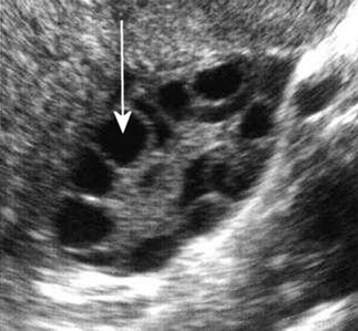
Figure 42.1 The cysts within this polycystic ovary contain watery fluid and appear anechoic (echo free).
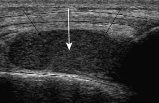
Figure 42.2 This haemorrhage into a joint returns many small bright echoes from the substances within it, such as blood cells and proteins. It is echogenic (echo producing).
Whenever an ultrasound beam reaches a boundary between two materials with different acoustic impedances, some of the beam will be reflected, and the remainder transmitted. The acoustic impedance, symbol Z, refers to the amount of opposition that a medium presents to sound waves trying to pass through it and is affected by the compressibility and density of the medium. The greater the acoustic impedance between two tissues, the greater is the amount of sound reflection at the boundary between them.
• Soft tissue/air interface – large Z difference=large reflection.
• Soft tissue/bone interface – large Z difference=large reflection (about 100%).
The acoustic impedances of body tissues can be seen in Table 42.2.
Table 42.2 Acoustic impedance (Z) values for air and body tissues
| MATERIAL OR TISSUE | ACOUSTIC IMPEDANCE (KG.M−2.S−1) |
|---|---|
| Air | 0.004 × 10⁶ |
| Fat | 1.34 × 10⁶ |
| Water | 1.48 × 10⁶ |
| Liver | 1.65 × 10⁶ |
| Blood | 1.65 × 10⁶ |
| Muscle | 1.71 × 10⁶ |
| Bone | 7.8 × 10⁶ |
Large Z differences return good strong echoes but will prevent sound waves from penetrating beyond the boundary to show deeper structures. For this reason it is almost (but not quite) technically impossible to see deep structures through the skull using diagnostic ultrasound in adults. The air-filled lungs and ribs also present barriers to ultrasound. Muscle/liver, muscle/fat and muscle/air boundaries reflect back about 2%, 10% and 99% of sound respectively. Good ultrasound images of deep structures result when there are moderate but not huge Z differences between tissues.
The process of reflection of sound at a boundary is illustrated in Figure 42.3. Dense objects such as gallstones reflect back large amounts of sound, due to the large acoustic impedance difference between themselves and surrounding substances. This may lead to the appearance of an acoustic shadow on an ultrasound scan. This takes the form of a dark echo-free band radiating out behind the stone, in a region where no sound has penetrated. An acoustic shadow can be seen in Figure 42.4.
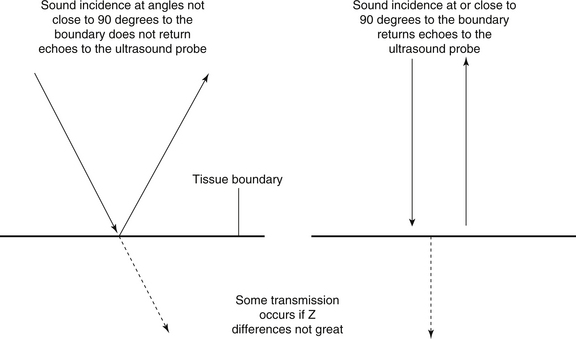
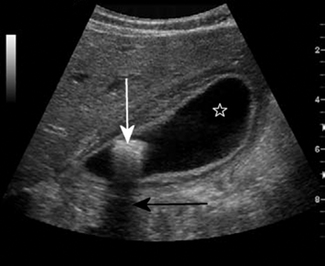
Figure 42.4 A gallstone (white arrow) is returning many echoes and has a bright hyperechoic appearance on its leading face. Behind this there is an acoustic shadow (black arrow) where no sound has been transmitted. There are also bright echoes at the boundary between the wall of the gall bladder and its contained fluid, which appears dark and anechoic (star).
An alternative effect, refraction, although important for visible light, is not a major process in diagnostic ultrasound and so sound reflections are much stronger than sound refractions at tissue boundaries. In the process of refraction, a wave carries on from one material to another – it isn’t reflected back. Refraction is an alteration in propagation direction (direction of travel) which occurs at a boundary between two materials in which the speed of the wave differs. The wave is bent ‘towards the normal’ if the new speed is slower than the original, and ‘away from the normal’ if the new speed is faster. The process of refraction at a boundary is shown in Figure 42.5.
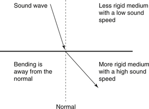
Figure 42.5 The process of refraction at a boundary between two media. In this case the sound is refracted away from the normal (the normal is at 90° to the boundary).
Although all electromagnetic radiations in a vacuum travel at the speed of light, c, which is about 299 792 000 metres per second (2.998 × 10⁸ m.s−1), visible light travels at slightly different speeds in different media. In water and glass, visible light travels at speeds of about 2.25 × 10⁸ m.s−1 and 1.98 × 10⁸ ms−1 respectively. The alteration in speed of light (and sound) at boundaries is part of the process of refraction and, in the case of light, explains the production of a rainbow spectrum in a glass prism, with different light wavelengths being refracted to different extents. X-rays have a much higher frequency and energy than visible light. As a result, although they do experience changes in speed in different media; this is to an infinitesimal degree of no practical significance. X-rays experience absorption and scattering in matter, rather than refraction and reflection, although diffraction effects can be seen in very low-energy X-rays whose wavelength is similar to the spacing between atoms in crystal structures.
Sound shares some properties with electromagnetic radiations, in that all of them can be considered as waves with a frequency, wavelength and amplitude. In all of these cases, the velocity of the wave (in metres per second) is equal to the frequency (in Hertz) multiplied by the wavelength (in metres).

A key difference between sound and electromagnetic waves is that sound is regarded as a longitudinal wave. This means that the oscillations of the wave (in this case, compressions and rarefactions in a medium) are in the direction of travel rather than at right angles to it. Figure 42.6 shows the process of sound transmission through a medium.
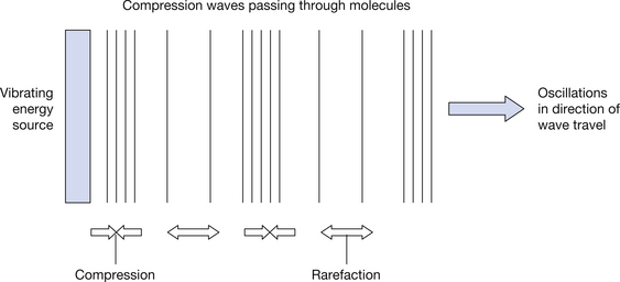
Figure 42.6 Passage of a longitudinal wave through a medium. The waves radiate out from the source, like ripples moving away from where a pebble has splashed in a pool.
Other examples of longitudinal waves include waves in slinky springs, ripples in a water tank, trucks shunting into each other on a rail track, a trick shot with a row of snooker balls!
The frequency of medical ultrasound is in the range of 2–20 MHz (megahertz). In medical ultrasound, low frequencies in this range penetrate deeper into the body but have a low resolution, while high sound frequencies can only penetrate a shallow depth in the body but have a high resolution. The term ultrasound means sound that is above the audible range of hearing for humans (the human range is roughly 20 Hz to 20 kHz).
Table 42.3 summarizes some key properties of sound, light and X-rays.
Table 42.3 Similarities and differences between sound, light and X-rays
| SOUND | VISIBLE LIGHT | X-RAYS |
|---|---|---|
| Velocity=fγ | Velocity=fγ | Velocity=fγ |
| Slow velocity | Velocity is light speed, c, in vacuum | Velocity is light speed, c, in vacuum |
| Velocity much affected by medium | Velocity slightly affected by medium | Velocity not affected by medium |
| Longitudinal waves | Transverse waves | Transverse waves |
| Vibrations in atoms and molecules | Photons (quanta) | Photons (quanta) |
| Mainly absorbed, reflected | Mainly absorbed, reflected, refracted | Mainly absorbed, scattered |
| Non-ionizing | Non-ionizing | Ionizing |
42.3 The doppler effect
When an object which is emitting sound approaches an observer at speed, the waves become ‘bunched-up’ and the frequency (or pitch) of the sound increases. Similarly if an object which is emitting sound moves away from an observer at speed, the waves become ‘drawn out’ and the frequency (or pitch) of the sound decreases. This effect is shown in Figure 42.7.
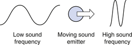
This principle has important clinical applications in diagnostic ultrasound, since the altered sound frequency of moving tissues, such as heart valves and flowing blood, can be used to determine their speed of movement relative to the ultrasound probe. In colour-coded Doppler imaging, motion towards the probe is traditionally depicted as red, while motion away from the probe is depicted as blue.
The Doppler effect can be observed when the speed of wave-emitting objects is significant relative to the speed of the waves. Doppler shift of light occurs in space when galaxies are moving away from us at tremendous speeds. At these high speeds, visible light becomes shifted towards the red end of the spectrum and this effect can be used to measure the expansion of the universe.
42.4 Production and application of ultrasound
An ultrasound transducer (probe) typically consists of an array of individual elements. Each element contains a piezoelectric crystal, typically made of ceramic material combinations of lead titanate (PbTiO3) and lead zirconate (PbZrO3). An alternating voltage applied across the crystal will cause it to flex and emit sound vibrations at an adjustable frequency. Also the crystal will generate an alternating voltage across itself in response to a returning sound wave, resulting in a signal. The crystal can be thought of as acting both as a sound speaker and a sound recorder. The elements of the transducer array can be focused to receive signal from shallow or deeper structures in the body.
The various modes of ultrasound scanning available include the following:
• A mode – amplitude modulated. Produces a graph plot whose height on the y-axis shows the strength of the echoes received from the reflective boundary and whose position on the x-axis shows the depth of the boundary. Can be used to show motion in structures such as heart valves, if the data are converted to an m mode (motion) trace where the position of a reflective boundary is plotted against time.
• B mode – brightness modulated. Produces a 2D anatomical slice through the body with a greyscale brightness based on the amplitude and frequency of reflected sound. This is the most common type of ultrasound scan and the most easy to interpret visually. The depth of the reflective structure (as with A mode scanning) is determined from the time it takes for the echo to return to the transducer.
• Doppler ultrasound – change in sound frequency indicates speed of tissue motion and may be plotted as a colour display plot. A spectral plot may be included, to indicate motion on the y-axis over time on the x-axis. Pulsed wave Doppler enables the operator to adjust the depth of tissue being visualized, by only accepting returning echoes with time lags in a particular range.
• Duplex scanning combines a Doppler scan with a B mode display which is used for localization purposes.
• Endoscopic ultrasound uses small intracavity transducers which can show the insides of structures like the oesophagus and blood vessels.
• 3D transducer arrays provide a 3D depiction of structures and are most popularly used to depict the fetus in utero.
Ultrasound imaging of tissue structures produces harmonic frequencies, which are multiples of the fundamental (or basic) returning sound frequency. For example, the 2nd harmonic is twice the frequency of the fundamental. Harmonics are of great importance to the tones of sound we hear in music. In ultrasound, filters can be used to separate out the 2nd harmonic, which, being of higher frequency, also provides greater resolution. Microbubble contrast agents in ultrasound include bubbles of gas just a few microns in size and are more compressible than surrounding substances. Thus, they return echoes and can be used to improve the visualization of blood vessels and tissues such as the liver. The microbubbles resonate and produce harmonic frequencies in response to ultrasound waves and this further improves depiction.
Some of the clinical strengths and weaknesses of ultrasound are summarised in Table 42.4.
Table 42.4 Features of clinical ultrasound
| STRENGTHS | WEAKNESSES |
|---|---|
| Inexpensive | Operator dependent |
| Quick | Images may be hard to interpret |
| Mobile | Suffers from image artefacts |
| Non-invasive | May be prone to giving ‘false positives’ |
| Can depict free fluid and aneurysms, e.g. in acute emergencies | Not good for deep structures |
| Can differentiate between solid and fluid structures | Cannot penetrate through bone or air |
| Can depict flow and motion | |
| Good for shallow structures |
The biological effects of ultrasound are mainly heat and cavitation. Cavitation occurs in oscillating gas bubbles that can be produced and then collapse in tissues. To reduce these effects on the developing fetus in utero, there are recommended restrictions on the power output, scan time and duty cycle (pulse length and repetition frequency) in pregnancy. Although some researchers have proposed that dyslexia, left-handedness and reduced birth weight can result from ultrasound use in pregnancy, these studies have not been verified and there is no proven long-term harm resulting from ultrasound.
In this chapter, you should have learnt the following:
• Medical ultrasound employs high-frequency sound waves which show boundaries between tissues by being reflected at them (see Sect. 42.2).
• Sound waves are unlike the other radiations used in radiography and require a medium for transmission (see Sect. 42.2).
• Reflections are strongest when there are sound transmission differences between tissues, but large differences may be unhelpful by preventing sound transmission to deeper structures (see Sect. 42.2).
• Doppler ultrasound provides information on the speed of moving tissues (see Sect. 42.3).