Chapter 10 Instrumentation and controls
INTRODUCTION
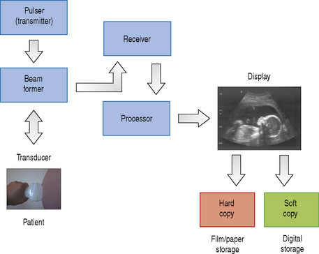
A diagnostic ultrasound machine consists of many components, each of which has a separate operation to perform. This starts with transmitting and receiving ultrasound signals which are then processed to form the images that we see on screen. The internal components that make up a typical ultrasound machine are listed below. Figure 10.1 illustrates the architecture of the components in a block diagram.
COMPONENTS OF A TYPICAL ULTRASOUND MACHINE
The Transducer
Diagnostic transducers are made from piezoelectric materials (see chapter on Transducers) and are able to convert electrical energy into ultrasound energy and vice versa. As a consequence of this they can act as a transmitter and receiver of ultrasound. They are able to produce beams which can be directed in various ways which are controlled by the ultrasound machine to improve image quality.
The Pulser
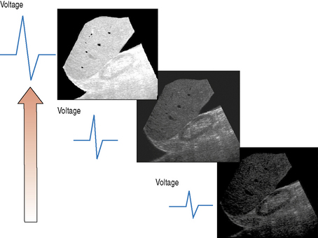
The pulser produces the electric voltage that drives the transducer. This driving voltage governs the output power of the ultrasound machine and can be adjusted by the operator through the power or output control. Changes in the applied voltage to the transducer changes the strength and intensity of the ultrasound beam, and affects the overall brightness of the B-mode image. The greater the applied voltage, the stronger the ultrasound pulse and the higher the pulse intensity. Figure 10.2 illustrates the effect that increasing the applied voltage has on the B-mode image. Increasing the applied voltage to the transducer increases the ultrasound pulse intensity, resulting in an increase in the overall brightness of the image.
Beam Former
The beam former controls the shape and direction of the ultrasound beam and the scanning patterns used to form the images that we see. This enables the operator to have indirect control of:
Receiver
The job of the receiver is to combat attenuation, i.e. the energy lost from the beam as it propagates through soft tissue. As a consequence of attenuation the returning echo amplitudes and intensities are decreased. Most of the energy is lost from the beam through absorption which is mainly converted into heat. The receiver applies amplification to the returning echoes to make them stronger and to enable them to be visualized. The ultrasound machine can compensate for the effects of attenuation by amplifying the received signals in two ways, using the overall gain and the time-gain compensation (TGC) controls.
Processor
The processor can be divided into two individual parts, each having very different tasks to fulfil, and consists of:
A simple block diagram of the signal processor is illustrated in Figure 10.3. The signal processor picks up the amplified signals from the receiver and carries out operations such as filtering, amplitude detection, and signal compression.
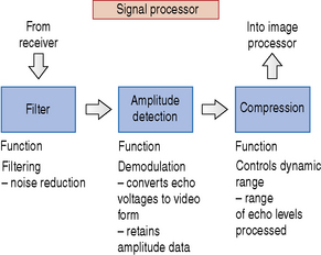
Filtering cleans up the signal, removing unwanted noise, and also controls the signal bandwidth (see chapter on Transducers). Amplitude detection performs a process of demodulation which means it converts the received signal voltages into video form, retaining the amplitude information required for B-mode imaging. Compression controls the dynamic range of the B-mode image (the number of shades of gray displayed in the image).
Once the signals have passed through the signal processor they are fed into the image processor. A block diagram of the image processor is illustrated in Figure 10.4. The image processor performs operations such as scan conversion which reformats the scan line data into two-dimensional images, i.e. either linear or sector form. The ability of the scan converter to rapidly process the thousands of scan line data received every second from the transducer enables real-time dynamic ultrasound imaging to be performed.

There is a range of processing performed on the image data prior to and following storage into memory before they are finally sent to the display. Functions such as edge enhancement are known as pre-processing functions because they are performed before being stored.
Image memory stores a number of sequentially acquired and processed static image frames every second which are rapidly sent to the display to provide dynamic real-time ultrasound. This process can be interrupted by activating the freeze control which stops any further acquisition and processing of data from the transducer. In freeze mode only one static image in the memory is displayed. The numerous frames of image data held and stored can be reviewed in turn using the machine’s cineloop control function.
The Display
Once the images have been processed they can either be displayed on a traditional cathode ray tube which is used in conventional televisions or be presented on a computer monitor or a flat panel screen. There are only two controls that can be adjusted on most displays, which are brightness and contrast. These can be set by the operator according to individual preference or ambient room lighting conditions.
Hard Copy and Soft Copy Storage
The images displayed on screen can be sent out to an external hard copy device such as radiographic film or thermal paper printers. Alternatively, the images, which can also consist of short cineloop review video clips, can be digitally stored on the machine’s hard disc or alternatively burnt to CD or DVD. Many ultrasound departments are linked into a picture archiving and communications system, more commonly known as PACS. This enables images such as X-rays and ultrasound scans to be stored electronically and viewed on any PACS display monitor around the hospital at the touch of a button.
SYSTEM CONFIGURATION - USE OF PRESETS
Many ultrasound machines provide the operator with a range of stored preconfigured control settings known as presets. Before starting any investigation the operator should select and initialize the specific preset which has been configured to automatically select various control parameters such as gain, depth, power, focus, etc., together with the most appropriate processing functions to optimize the image performance of the ultrasound system. There are a number of different presets which can be selected by the operator for each type of clinical examination whether it be, for example, liver, pelvis, obstetric, abdominal, or vascular. The ultrasound system can also store additional presets for different users; each stored preset can be selected with a single keystroke.
Despite the inclusion of system configured presets in most current ultrasound equipment it is important for the operator to have an understanding of the function of each manual control, because many of these preset modes will require further manual manipulation throughout the scanning procedure. Patient body habitus will vary significantly, resulting in a requirement for changes to the equipment controls throughout the examination.
FUNCTION OF ULTRASOUND CONTROLS
Image Controls
A large number of controls are available to be used on most ultrasound equipment but the more important and most frequently used controls are discussed below.
Output power
The output power of an ultrasound machine is determined by the pulser which produces the electric voltage that drives the transducer. The output power is automatically set for each preset mode and can be manually manipulated through the power or output control. Ultrasound machines’ output powers are limited, and should not exceed 720 mWcm−2 specifically for safety reasons (see chapter on Ultrasound safety).
The effect of increasing the output is to increase the amplitude and intensity of emitted ultrasound pulses which in turn increases the size of the returning signals. Improving the signal strength of returning echoes improves the clarity and detail of structures within the B-mode image. The effect of increasing the output power is demonstrated in Figure 10.2 which shows that the higher the output power, the brighter the overall B-mode image.
However, increasing the output power causes the patient to be exposed to more ultrasound energy which could increase the risk of causing any possible harmful effects that are more likely to affect sensitive tissues such as rapidly developing cells found in embryo, fetus, and neonate. The alternative and safer option rather than increasing the output power is to amplify the received signals using the machine’s gain and/or TGC controls. This minimizes exposure while improving the image quality.
Overall gain
Overall receiver gain provides uniform amplification of all the received signals regardless of depth, and affects the brightness of the overall image. The operation of the gain is to compensate for the loss of energy through attenuation as the beam propagates through the patient.
There is no ‘absolute’ or ‘correct’ setting. The gain will require adjustments throughout the examination and will vary with each individual patient according to the organ or vessel being scanned or to the body habitus of the patient. This will involve increasing the level of the gain for scanning deeper structures and decreasing it when scanning superficial structures. However, there is a limit to how much the received signals can be amplified which is governed by the level of noise within the signal.
Amplifying the signal strength also amplifies the level of background noise within the signal, which becomes more significant as the levels of amplification increase to the point where the level of the background noise in the signal is greater than that of the received signal. The depth at which this occurs is known as the penetration depth. When background noise is visualized this is the point to stop increasing the gain and to increase the output power if safe to do so.
Time-gain compensation (TGC)
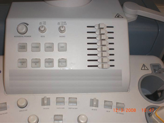
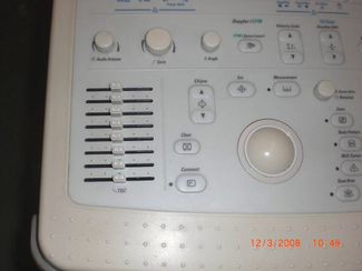
The TGC is similar to the overall gain inasmuch as they both compensate for the effects of attenuation. Attenuation causes weaker signals to be received from structures that lie deeper than those which lie closer to the face of the transducer. The TGC can compensate for this loss of signal strength so that equal amplitudes can be displayed from all depths within the scan plane as the same brightness on the image. This is simply achieved by applying a variable gain to the received signals so that signals returning later are amplified more than those previously received. The TGC does this through a number of horizontal slider controls as shown in Figure 10.5. Their relative position governs the amount of gain applied to the received signals from various depths within the scan plane. The net result produces received signals of similar amplitude and displayed brightness over depth.
The processes involved with TGC of received signals are illustrated in Figure 10.6.
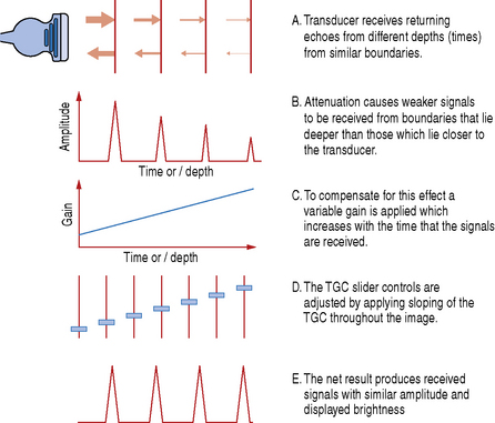
Fig. 10.6 Illustrating the processes involved with TGC of received signals
(After Thrush & Hartshorne 2005.)
Depth
The depth control changes the maximum scanning range viewed on screen. The ultrasound machine determines depth indirectly by measuring the time it takes for a pulse to return. The system has to wait to receive all the returning echoes along each scan line for a selected depth before sending another. As the depth control is increased the time it takes for a pulse to return to the transducer also increases. This time factor imposes an upper limit to the time interval between consecutive transmit pulses known as the pulse repetition frequency (PRF). Changes in the depth changes the maximum pulse repetition rate which affects the frame rate.
Increasing the depth decreases the system’s PRF which decreases the number of image frames that can be displayed per second (fps).
Focus
The focus determines the depth at which the ultrasound beam is focused and creates the best possible resolution at that depth.
The focal position is usually displayed by a symbol or vertical bar or bracket alongside the display of the B-mode image. The focal zone should be positioned at or just below the level of interest within the B-mode image. The operator is able to activate more than one focal zone, sometimes as many as five, however for each additional focal zone another pulse must be sent along the same scan line. As a consequence of this, the number of frames of image data per second (fps) is reduced, resulting in a slower frame rate and the images appearing disjointed.
The number of focal zones is related to the frame rate and is illustrated in the example below:
Freeze and cineloop
Activating the freeze button stops any further acquisition and processing of data from the transducer. Once frozen the ultrasound machine displays the last acquired image which is held in image memory. Image memory is able to store many frames of image data which can be individually reviewed in turn using the cineloop control function. The actual number of stored frames in the image memory will vary according to the frame rate being used.
Sector width
The sector width, also referred to as the sector angle, is important in determining the frame rate at a given depth. The size of the sector width or angle can be reduced by the operator and is as illustrated in Figure 10.7.
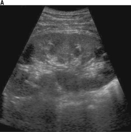
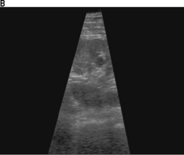
Fig. 10.7 Illustrating sector width. a) B-mode image for a given depth, sector width and line density determines the frame rate. b) Image with a reduced sector width
B-mode images are made up of a number of adjacent scan lines; there can be many hundreds of scan lines used to form one image and the number of scan lines used is known as the line density. A sector width for a given depth and line density determines the frame rate and is seen in Figure 10.7a.
Reducing the sector width as seen in Figure 10.7b can bring about improvements to the overall frame rates and/or image resolution.
At a given depth, reducing the sector width means that fewer scan lines are required to form an image. This reduces the time needed to build up an image, resulting in higher frame rates. These high frame rates are required when imaging the heart, for example, and this technique of improving the overall frame rate is used especially when scanning the fetal heart in obstetrics.
Alternatively, reducing the sector width can bring about improvements to image resolution if the number of scan lines within this reduced sector is maintained, i.e. using thinner scan lines. This brings about no improvements to frame rates (they remain unchanged), but the increased line density increases the spatial resolution, namely lateral resolution.
The benefits of reducing the sector width are summarized in Table 10.1.
Table 10.1 Summarizing the benefits brought about by reducing the sector width
| Benefit | Result | |
|---|---|---|
| Reducing the size of the sector width | – increases scan line density – more scan lines over the same area | – better detail – increased image resolution |
| – fewer scan lines to process – increases frame rate | – increased temporal resolution |
Zoom
If the region within the B-mode image is small or very deep the operator can use the zoom control to magnify an area of interest on the screen. The machine often allows the operator to adjust the size and position of the region of interest. There are two forms of zoom, read zoom and write zoom.
Read zoom simply magnifies the image, bringing about no improvements to the quality of the image. Using read zoom is similar to looking at news print very close up or using the digital zoom facility on modern digital cameras.
Real zoom, also known as write zoom, increases the ultrasound information content within the image, i.e. improves image resolution by increasing the scan line density and the number of pixels per square centimeter. The effect is similar to using a camera’s optical zoom function.
On some machines it can be difficult to determine if the zoom facility is either read or write.
Dynamic range/log compression
Dynamic range refers to the way that the gray scale information is compressed into a usable range for display on the monitor. A broader or wide dynamic range yields more shades of gray, while a smaller or narrow dynamic range results in a more black and white appearance of the image. Figure 10.8 illustrates the effect that increasing the dynamic range has on the ultrasound image.
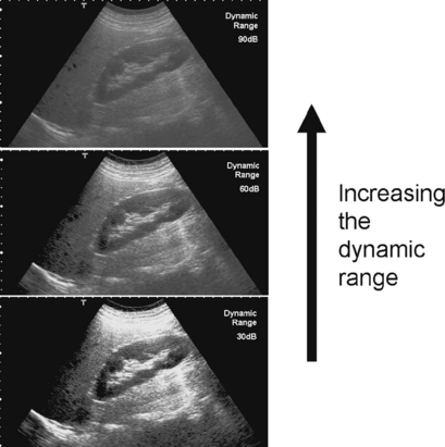
Fig. 10.8 Demonstrating the effect that increasing the dynamic range has on the overall ultrasound image
Since the range of signal amplitudes which are detected is so large, a decibel scale is used (dB).The dynamic range in decibels (dB) refers to the amount that the signal is compressed and expressed as the ratio of the largest to the smallest signal that can be visualized (white and black respectively).
For example, 60 dB represents a ratio of 1 000 000:1. The displayed dynamic range will affect the echo/gray scale assignment. A dynamic range of 40 dB (10 000:1 ratio) gives a highly contrasted image (see Fig. 10.8) that may be better for visualizing the walls of vessels, for example. Here, we are not interested in differentiating between a wide range of gray levels as blood appears black and vessel walls appear bright white. A dynamic range of 60 dB gives a softer image that may prove better for visualizing subtle differences within and between tissues, for example when scanning the liver as illustrated in Figure 10.8.
MEASUREMENTS
Measurement of key parameters within an ultrasound image is an essential part of interpreting ultrasound scans and aids with differentiating normal anatomy from pathology, monitoring fetal growth patterns, and are used to estimate due dates for delivery. Ultrasound machines are able to take a variety of measurements from frozen static B-mode images which include: