Introduction to Sectional Anatomy
Sectional anatomy has had a long history. Beginning back as early as the sixteenth century, the great anatomist and artist, Leonardo da Vinci, was among the first to represent the body in anatomic sections. In the following centuries, numerous anatomists continued to provide illustrations of various body structures in sectional planes to gain greater understanding of the topographical relationships of the organs. The ability to see inside the body for medical purposes has been around since 1895, when Wilhelm Conrad Roentgen discovered x-rays. Since that time, medical imaging has evolved from the static, 2-dimensional (2D) image of the first x-ray to the 2D cross-section image of computed tomography (CT) and finally to the 3-dimensional (3D) imaging techniques used today. These changes warrant the need for medical professionals to under stand and identify human anatomy in both 2D and 3D images.
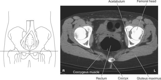
Sectional anatomy emphasizes the physical relationship between internal structures. Prior knowledge of anatomy from drawings or radio graphs may assist in understanding where specific structures are located on a sectional image. For example, it may be difficult to recognize all the internal anatomy of the pelvis in cross section, but by identifying the femoral head on the image, it will be easier to recognize soft tissue structures adjacent to the hip in the general location of the slice (Figure 1.1).
ANATOMIC POSITIONS AND PLANES
For our purposes, sectional anatomy encompasses all the variations of viewing anatomy as a 2D slice taken from an arbitrary angle through the body while in anatomic position.
In anatomic position the body is standing erect, face and toes pointing forward, and arms at the side with the palms facing forward. Sectional images are acquired and displayed according to one of the four fundamental anatomic planes that pass through the body (Figure 1.2). The four anatomic planes are defined as follows:
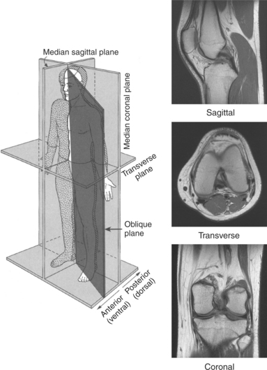
1. Sagittal plane: a vertical plane that passes through the body, dividing it into right and left portions
2. Coronal plane: a vertical plane that passes through the body, dividing it into anterior (ventral) and posterior (dorsal) portions
3. Axial (transverse) plane: a horizontal plane that passes through the body, dividing it into superior and inferior portions
4. Oblique plane: a plane that passes diagonally between the axes of two other planes
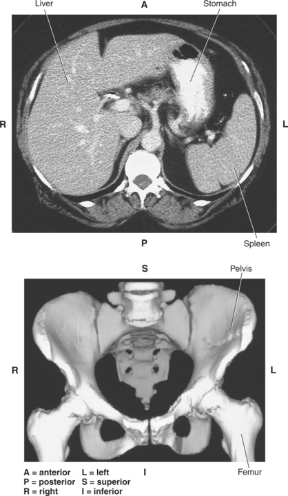
Medical images of sectional anatomy are, by convention, displayed in a specific orientation. Images are viewed with the right side of the image corresponding to the viewer’s left side (Figure 1.3).
TERMINOLOGY AND LANDMARKS
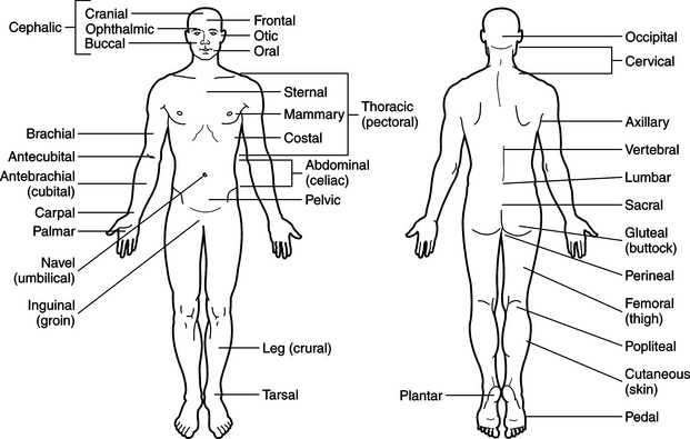
Directional and regional terminology is used to help describe the relative position of specific structures within the body. Directional terms are defined in Table 1.1, and regional terms are defined in Table 1.2 and demonstrated in Figure 1.4.
TABLE 1.1
| DIRECTION | DEFINITION |
| Superior | Above; at a higher level |
| Inferior | Below; at a lower level |
| Anterior/ventral | Toward the front or anterior surface of the body |
| Posterior/dorsal | Toward the back or posterior surface of the body |
| Medial | Toward the midsagittal plane |
| Lateral | Away from the midsagittal plane |
| Proximal | Toward a reference point or source within the body |
| Distal | Away from a reference point or source within the body |
| Superficial | Near the body surface |
| Deep | Farther into the body and away from the body surface |
| Cranial/cephalic | Toward the head |
| Caudal | Toward the feet |
| Rostral | Toward the nose |
| Ipsilateral | On the same side |
| Contralateral | On the opposite side |
| Thenar | The fleshy part of the hand at the base of the thumb |
| Volar | Pertaining to the palm of the hand or flexor surface of wrist |
| Palmar | The front or palm of the hand |
| Plantar | The sole of the foot |
TABLE 1.2
| DIRECTION | DEFINITION |
| Abdominal | Abdomen |
| Antebrachial | Forearm |
| Antecubital | Front of elbow |
| Axillary | Armpit |
| Brachial | Upper arm |
| Calf | Lower posterior portion of leg |
| Carpal | Wrist |
| Cephalic | Head |
| Cervical | Neck |
| Costal | Ribs |
| Cubital | Posterior surface of elbow area of the arm |
| Femoral | Thigh |
| Flank | Side of trunk adjoining the lumbar region |
| Gluteal | Buttock |
| Inguinal | Groin |
| Lumbar | Lower back between the ribs and hips; loin |
| Mammary | Upper chest or breast |
| Occipital | Back of the head |
| Ophthalmic | Eye |
| Pectoral | Upper chest or breast |
| Pelvic | Pelvis |
| Perineal | Perineum |
| Plantar | Sole of foot |
| Popliteal | Back of knee |
| Sacral | Sacrum |
| Sternal | Sternum |
| Thigh | Upper portion of leg |
| Thoracic | Chest |
| Umbilical | Navel |
| Vertebral | Spine |
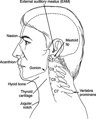
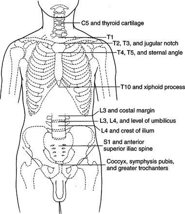
External Landmarks
External landmarks of the body are helpful to identify the location of many internal structures. The commonly used external landmarks are shown in Figures 1.5 and 1.6.
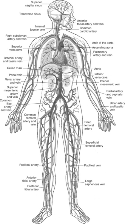
Internal Landmarks
Internal structures, in particular vascular structures, can be located by referencing them to other identifiable regions or locations such as organs or the skeleton (Figure 1.7and Table 1.3).
TABLE 1.3
| LANDMARK | LOCATION |
| Aortic arch | 2.5 cm below jugular notch |
| Aortic bifurcation | L4-L5 |
| Carina | T4-T5, sternal angle |
| Carotid bifurcation | Upper border of thyroid cartilage |
| Celiac trunk | 4 cm above transpyloric plane (Figure 1.10) |
| Circle of Willis | Suprasellar cistern |
| Common iliac vein bifurcation | Upper margin of sacroiliac joint |
| Conus medullaris | T12 to L1, L2 |
| Heartapex | 5th intercostal space, left midclavicular line |
| Heartbase | Level of 2nd and 3rd costal cartilages behind sternum |
| Inferior mesenteric artery | 4 cm above bifurcation of abdominal aorta |
| Inferior vena cava | L5 |
| Portal vein | Posterior to pancreatic neck |
| Renal arteries | Anterior to L1, inferior to superior mesenteric artery |
| Superior mesenteric artery | 2 cm above transpyloric plane |
| Thyroid gland | Thyroid cartilage |
| Vocal cords | Midway between superior and inferior border of thyroid cartilage |
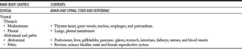
BODY CAVITIES
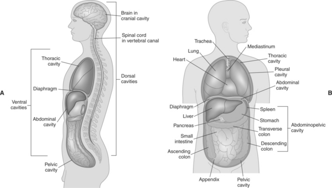
The body consists of two main cavities: the dorsal and ventral cavities. The dorsal cavity is located posteriorly and includes the cranial and spinal cavities. The ventral cavity, the largest body cavity, is subdivided into the thoracic and abdomino pelvic cavities. The thoracic cavity is further subdivided into two lateral pleural cavities and a single, centrally located cavity called the mediastinum. The abdominal cavity can be sub divided into the abdominal and pelvic cavities (Figure 1.8, A and B). The structures located in each cavity are listed in Table 1.4.
ABDOMINAL AND PELVIC DIVISIONS
The abdomen is bordered superiorly by the diaphragm and inferiorly by the superior pelvic aperture (pelvic inlet). The abdomen can be divided into quadrants or regions. These divisions are useful to identify the general location of internal organs and provide descriptive terms for the location of pain or injury from a patient’s history.
Quadrants
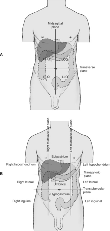
The midsagittal plane and transverse plane intersect at the umbilicus to divide the abdomen into four quadrants (Figure 1.9, A):
For a description of the structures located within each quad rant, see Table 1.5.
TABLE 1.5
Organs Found within Abdominopelvic Quadrants
| QUADRANT | ORGANS |
| Right upper quadrant (RUQ) | Right lobe of liver, gallbladder, right kidney, portions of stomach, small and large intestines |
| Left upper quadrant (LUQ) | Left lobe of liver, stomach, tail of the pancreas, left kidney, spleen, portions of large intestines |
| Right lower quadrant (RLQ) | Cecum, appendix, portions of small intestine, right ureter, right ovary, right spermatic cord |
| Left lower quadrant (LLQ) | Most of small intestine, portions of large intestine, left ureter, left ovary, left spermatic cord |
Regions
The abdomen can be further divided by four planes into nine regions. The two horizontal planes are the transpyloric and transtubercular planes. The transpyloric plane is found midway between the xiphisternal joint and the umbilicus, passing through the inferior border of the L1 vertebra. The trans tubercular plane passes through the tubercles on the iliac crests, at the level of the L5 vertebral body. The two sagittal planes are the midclavicular lines. Each line runs inferiorly from the midpoint of the clavicle to the midinguinal point (Figure 1.9, B). The nine regions can be organized into three groups:
IMAGE DISPLAY
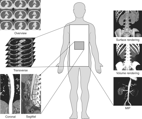
The following section is intended to introduce the reader to the various methods with which sectional images will be displayed within the text (Figure 1.10). For a more in-depth discussion of the topics, refer to the reference list at the end of the chapter.
Gray Scale
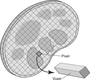
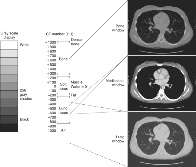
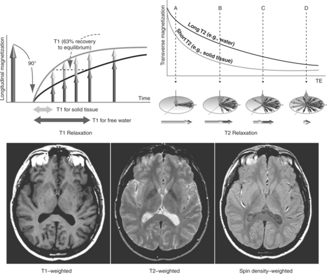
Each digital image can be divided into individual regions called pixels or voxels that are then assigned a numerical value corre sponding to a specific tissue property of the structure being imaged (Figure 1.11). The numerical value of each voxel is assigned a shade of gray for image display. In CT, the numerical value (CT number) is referenced to a Hounsfield unit (HU), which represents the attenuating properties or density of each tissue. Water is used as the reference tissue and is given a value of zero. Any CT number greater than zero will represent tissue that is denser than water and will appear in progressively lighter shades of gray to white. Tissues with a negative CT number will appear in progressively darker shades of gray to black. In magnetic resonance (MR), the gray scale represents the specific tissue relaxation properties of T1, T2, and relative spin density. The gray scale in MR images can vary greatly because of inherent tissue properties and can appear dif ferent with each patient and across series of images.
The appearance of each digital image can be altered to include more or fewer shades of gray by adjusting the gray scale, a process called windowing. Windowing is used to optimize visualization of specific tissues or lesions. Window width (WW) is the parameter that allows for the adjustment of the gray scale (number of shades of gray), and window level (WL) basically sets the density of the image (Figures 1.12 and 1.13).
Multiplanar Reformation and 3D Imaging
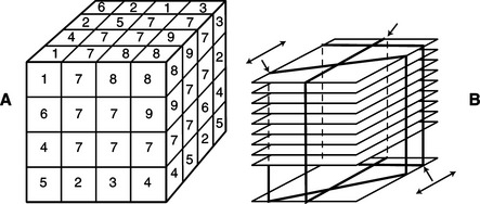
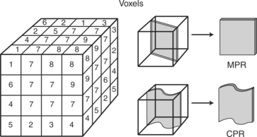
Several postprocessing techniques can be applied to the original 2D digital data that will provide additional 3D information for the physician. All current post-processing techniques depend on creating a stack of digital data from the original 2D images, which then results in a cube of digital information (Figure 1.14, A and B).
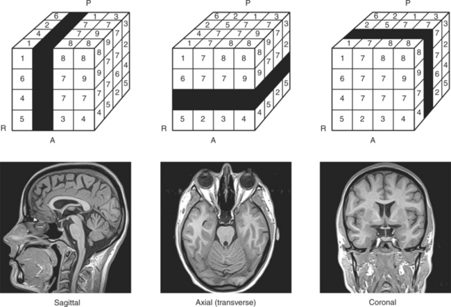
Multiplanar Reformation (Reformat) (MPR)
Images reconstructed from data obtained along any projection through the cube result in a sagittal, coronal, transverse, or oblique image (see Figure 1.10; Figure 1.15).
Curved Planar Reformation (Reformat) (CPR)
Images are reconstructed from data obtained along an arbi trary curved projection through the cube (Figure 1.16). All 3D algorithms use the principle of ray tracing in which imaginary rays are sent out from a camera viewpoint. The data are then rotated on an arbitrary axis, and the imaginary ray is passed through the data in specific increments. Depending on the method of reconstruction, unique information is projected onto the viewing plane (Figure 1.17).
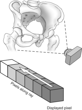
Shaded Surface Display (SSD)
A ray from the camera’s viewpoint is directed to stop at a particular user-defined threshold value. With this method, every voxel with a value greater than the selected threshold is rendered opaque, creating a surface. That value is then projected onto the viewing screen (see Figure 1.10; Figure 1.18).
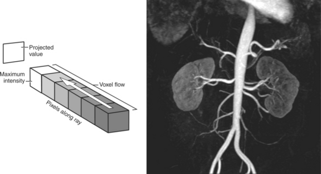
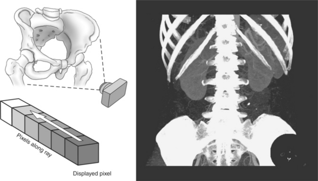
Maximum Intensity Projection (MIP)
A ray from the camera’s viewpoint is directed to stop at the maximum voxel value. With this method, only the brightest voxels will be mapped into the final image (Figure 1.19).
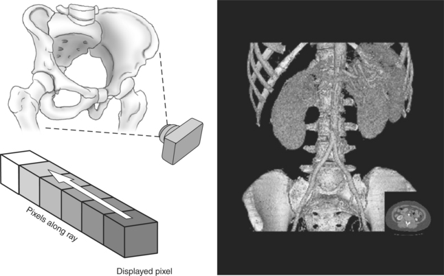
Volume Rendering (VR)
The contributions of each voxel are summed along the course of the ray from the camera’s viewpoint. The process is repeated numerous times in order to determine each pixel value that will be displayed in the final image (Figure 1.20).
Ballinger, PW. Radiographic positions and radiologic procedures, ed 10. St. Louis: Mosby, 2003.
Benson, HJ, Gunstream, SE, et al. Anatomy and physiology laboratory textbook, ed 4. Dubuque, IA: Wm. C. Brown, 1988.
Calhoun, PS, Kuszyk, BS, Heath, DG, et al. Three-dimensional volume rendering of spiral CT data: Theory and method. RadioGraphics. 1999;19:745.
Curry, RA, Tempkin, BB. Ultrasonography: An introduction to normal structure and functional anatomy, ed 2. St. Louis: Saunders, 2004.
Hofer, M. CT teaching manual. New York: Thieme Medical Publishers, 2000.
Moore, KL. Clinically oriented anatomy, ed 3. Baltimore: Williams & Williams, 1992.
Seeram, E. Computed tomography; physical principle, clinical applications, and quality control, ed 2. Philadelphia: Saunders, 2001.
Todd, EM. The neuroanatomy of Leonardo da Vinci. Park Ridge, IL: American Association of Neurological Surgeons, 1991.
Udupa, JK. Three-dimensional visualization and analysis methodologies: A current perspective. RadioGraphics. 1999;19:783.
White, M. Leonardo: the first scientist. New York: St. Martin’s Press, 2000.