Movement diagram theory and compiling a movement diagram
Appendix 1 remains as it was presented by Geoff Maitland in the 3rd edition of this book (1991). However, in view of contemporary developments arising from research and peer review of this subject, it was felt necessary by the current authors to add a contemporary perspective. What is clear is that movement diagrams remain a valuable tool for both current and developing clinical practice (Chesworth et al. 1998).
A contemporary perspective on defining resistance, grades of mobilization and depicting movement diagrams
Petty et al. (2002) in their peer review article ‘Manual examination of accessory movement-seeking R1’ have rightly challenged the long-held belief that for an asymptomatic joint, the resistance first felt by the therapist (R1) when the joint is moved passively occurs towards the end of the range. R1 is considered to be at the transitional point between the toe and linear regions of a load displacement curve (Lee & Evans 1994) (Fig. A1.1).
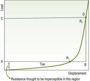
Figure A1.1 Relationship of movement diagram (ABCD) to load-displacement curve. Reproduced by kind permission from Petty et al. (2002).
Petty et al. (2002) used a spinal assessment machine which applied a posteroanterior force to the L3 spinous process whereby resistance was found to commence at the beginning of the range, the curve ascending as soon as the force was applied (Fig. A1.2).
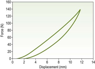
Figure A1.2 Typical force-displacement curve of a central PA applied to L3 obtained using the spinal assessment machine. The left-hand curve is loading and the right hand curve is unloading curve. Reproduced by kind permission from Petty et al. (2002).
The suggestions, therefore, are that there is no clear transition point between the toe and linear regions, this having previously been to the point of definition of R1. The lack of definite transition may explain the poor reliability of therapists in judging the onset of resistance to passive movement (R1) (Latimer et al. 1996).
Petty et al. (2002) suggest that R1 should be depicted as early as A on the movement diagram, A being the starting point of the range of movement. The consequence of this would be to call into question the accuracy of the resistance-based defined treatment grades of mobilization/manipulation (grades I–V) resulting in the loss of grades I and II and limiting the definitions to grades III and IV.
After due consideration of the case presented by Petty et al. (2002), the authors of this edition of Maitland's Peripheral Manipulation have proposed a reappraisal of the following:
1. The retention of grades I and II in the context of the redefinition of R1
The authors, therefore, are minded that such a reappraisal may affect the future direction of qualitative or quantitative research into movement diagrams, particularly in relation to the reliability of therapists' definition of R1 and the accurate calibration of treatment grades of mobilization and manipulation.
Redefining grades of mobilization
When a joint is moved passively (accessory or physiological, vertebral or peripheral) a variety of resistances are encountered, for example:
• The soft, immediate resistance to movement which fits to the laws of physics
• A firmer resistance to movement when the joint is nearing its end of range or its impaired limit (a stiff joint)
• The through-range resistance encountered when arthritic joints are moved with their joint surfaces squeezed together
The original resistance-defined grades of mobilization/manipulation (Maitland 1991) relate to resistance (R) being defined in terms of spasm-free resistance (stiffness) or hard and soft end-feel in the ideal or normal joint (Maitland 1992).
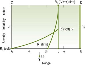
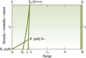
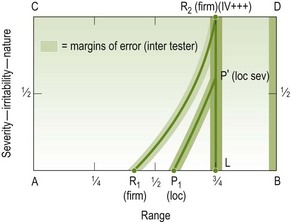
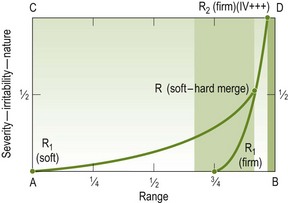
From the authors' viewpoint, therefore, the reference to resistance refers to the firmer resistance felt when a joint is nearing its end range or impaired limit (Fig. A1.3), rather than the soft resistance to movement which is felt immediately the joint is moved. It is clear that this definition of resistance can also be related to the resistance encountered due to protective involuntary muscle spasm (Fig. A1.4).
If such an argument is valid – and it may not be – then the grading system I, II, III, IV and V can still be retained but redefined as follows:
• Grade I – a small amplitude movement at the beginning of the available range where there is soft resistance but no firm resistance (a note should also be made that A is the starting point of the movement and can be varied according to where the start of the movement needs to be for best effects).
• Grade II – a large amplitude movement performed within the available range where there is soft resistance but no firm resistance.
• Grade III – a large amplitude movement performed into firm resistance or up to the limit of the available range.
• Grade IV – a small amplitude movement performed into firm resistance or up to the limit of the available range.
• Grade V – a small amplitude high velocity thrust performed usually, but not always, at the end of the available range.
Redefining resistance
Resistance (R1), in this context, would be redefined as follows:
• R1 (soft) – the onset of resistance encountered at the immediate moment that movement commences. Minimal; may even be imperceptible.
• R1 (firm) – the onset of resistance encountered due to: stiffness, the joint surfaces being squeezed together and moved, the hard and soft end-feel of a normal joint, protective involuntary muscle spasm (S1 would be the qualifying term in this case) or voluntary holding.
Movement diagram: parameters of reliability
In view of the low intertherapist reliability in detecting the relevant reference points and measurable parameters of a movement diagram, the authors suggest a redefining of some of these parameters. Maitland (1991) depicts B as a thickened point to account for the variation in the therapist's judgement of the end of the normal average range of passive movement. This should be extended to other reference points and parameters of measurement so that margins of error can be accounted for and clinical variations between individual therapist's perceptions can be recognized. Therefore:
• A still remains a fixed starting point but can be varied (all movements have a definite starting point)
• B has already been recognized as a thickened line
• R1 (soft) is easy to represent because it can be assumed its onset corresponds to the start of the movement at A
• R1 (firm) should be represented as a thickened line as is B in order to account for the margins of error in the individual perceptions of the onset of firm resistance
• L being the limit of impaired range should also be a thickened line to take account of the margins of error encountered in determining the limit of the impaired movement by P2, R2 or S2
• The lines P1 to P2 (P′), R1 to R2 (R′) (soft or firm) and S1 to S2 (S′) should all be depicted with margins of error to account for individual variations in their perception.
Figures A1.5 and A1.6 show the representation of such natural variations on movement diagrams.
The movement diagram: a teaching aid, a means of communication and self-learning
Geography would be incomprehensible without maps. They've reduced a tremendous muddle of facts into something you can read at a glance. Now I suspect … economics [read passive movement] is fundamentally no more difficult than geography except it's about things in motion. If only somebody would invent a dynamic map.
The movement diagram is intended solely as a teaching aid and a means of communication. When examining, say, a posteroanterior movement of the acromio-clavicular joint produced by pressure on the clavicle, newcomers to this method of examining will find it difficult to know what they are feeling. However, the movement diagram makes them analyse the movement in terms of range, pain, resistance and muscle spasm. Also, it makes them analyse the manner in which these factors interact to affect the movement.
Movement diagrams (and also the grades of movement) are not necessarily essential to using passive movement as a form of treatment. However, they are essential to understanding the relationship that the various grades of movement have to a patient's abnormal joint signs. Therefore, although they are not essential for a person to be a good manipulator, they are essential if the teaching of the whole concept of manipulative treatment is to be done at the highest level.
Movement diagrams are essential when trying to separate the different components that can be felt when a movement is examined. They therefore become essential for either teaching other people, or for teaching one's self and thereby progressing one's own analysis and understanding of treatment techniques and their effect on symptoms and signs.
The components considered in the diagram are pain, spasm-free resistance (i.e. stiffness) and muscle spasm found on joint examination, their relative strength and behaviour in all parts of the available range and in relation to each other. Thus the response of the joint to movement is shown in a very detailed way. The theory of the movement diagram is described in this appendix by discussing each component separately at first (for the practical compilation of a diagram for one direction of movement of one joint in a particular patient, see ‘Compiling a movement diagram’ below).
Each of the above components is an extensive subject in itself and it should be realized that discussion in this appendix is deliberately limited in the following ways:
• The spasm referred to is protective muscle spasm secondary to joint disorder
• Spasticity caused by upper motor neurone disease and the voluntary contraction of muscles is excluded.
Frequently this voluntary contraction is out of all proportion to the pain experienced yet in very direct proportion to the patient's apprehension about the examiner's handling of the joint. Careless handling will provoke such a reaction and thereby obscure the real clinical findings. Resistance (stiffness) free of muscle spasm is discussed only from the clinical point of view, i.e. discussion about the pathology causing the stiffness is excluded.
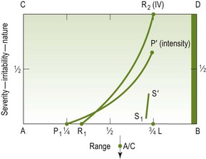
A movement diagram is compiled by drawing graphs for the behaviour of pain, physical resistance and muscle spasm, depicting the position in the range at which each is felt (this is shown on the horizontal line AB) and the intensity, nature or quality of each (which is shown on the vertical line AC) (Fig. A1.7).
The baseline AB represents any range of movement from a starting position at A to the limit of the average normal passive range at B, remembering that when examining a patient's movement of any joint, it is only considered normal if firm proportionate overpressure may be applied without pain. It makes no difference whether the movement depicted is large or small, whether it involves one joint or a group of joints working together, or whether it represents 2 mm of posteroanterior movement or 180° of shoulder flexion.
Because of soft-tissue compliance, the end of range of any joint (even ‘bone to bone’) will have some soft tissue component, physiological or pathological. Thus the range of the ‘end of range’ (B) will be a moveable point, or have a depth of position on the range line. To locate halfway through the range of the ‘end of range’ as a grade IV and to fit in either side of it a plus sign (1) and a minus sign (2) allows the depiction of the force with which this ‘end of range’ point is approached (Edwards, A., unpublished observations).
Point A, the starting point of the movement, is also variable: its position may be the extreme of range opposite B or somewhere in mid-range, whichever is more suitable for the diagram. For example, if shoulder flexion is the movement being represented and the pain or limitation occurs only in the last 10° of the range, the diagram will more clearly demonstrate the behaviour of the three factors if the baseline represents the last 20° rather than 90° of flexion. For the purpose of clarity, position A is defined by stating the range represented by the baseline AB. In the above example, if the baseline represents 90°, A must be at about 90°; similarly, if the baseline represents 20°, position A is with the arm 20° short of full flexion (assuming of course that the range of flexion is 180°).
As the movement diagram is used to depict what can be felt when examining passive movement, it must be clearly understood that point B represents the extreme of passive movement, and that this lies variably, but very importantly, beyond the extreme of active movement.
The vertical axis AC represents the quality, nature or intensity of the factors being plotted; point A represents complete absence of the factor and point C represents the maximum quality, nature or intensity of the factor to which the examiner is prepared to subject the person. The word ‘maximum’ in relation to ‘intensity’ is obvious: it means point C is the maximum intensity of pain the examiner is prepared to provoke. ‘Maximum’ in relation to ‘quality’ and ‘nature’ refers to two other essential parts. They are:
1. Irritability – when the examiner would stop the testing movement when the pain was not necessarily intense but when it was assessed that if the movement was continued into greater pain there would be an exacerbation or latent reaction.
2. Nature – when P1 represents the onset of, say, scapular pain, but as the movement is continued the pain spreads down the arm. The examiner may decide to stop when the provoked pain reaches the forearm.
Thus meaning of ‘maximum’ in relation to each component is discussed again later.
The basic diagram is completed by vertical and horizontal lines drawn from B and C to meet at D (Fig. A1.8).
Pain
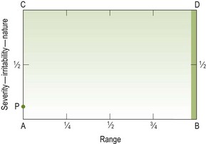
The initial fact to be established is whether the patient has any pain at all and, if so, whether it is present at rest or only on movement. To begin the exercise it is assumed that the patient only has pain on movement.
The first step is to move the joint slowly and carefully in the range being tested, asking the patient to report immediately when any discomfort is felt. The position at which this is first felt is noted.
The second step consists of several small oscillatory movements in different parts of the pain-free range, gradually moving further into the range up to the point where pain is first felt, thus establishing the exact position of the onset of the pain. There is no danger of exacerbation if:
The point at which this occurs is called P1 and is marked on the baseline of the diagram (Fig. A1.9).
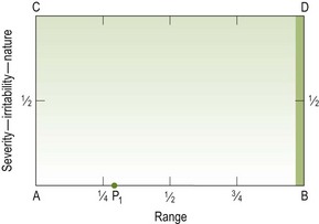
Thus there are two steps establishing P1:
If the pain is reasonably severe then the point found with the first single slow movement will be deeper in the range than that found with oscillatory movements. Having thus found where the pain is first felt with a slow movement, the oscillatory test movements will be carried out in a part of the range that will not provoke exacerbation.
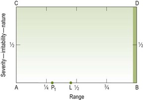
L (1 of 3) where (L 5 limit of range)
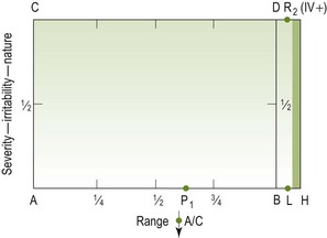
The next step is to determine the available range of movement. This is done by slowly moving the joint beyond P1until the limit of the range is reached. This point is marked on the baseline as L (Fig. A1.10).
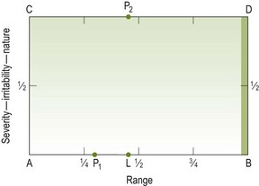
L (2 of 3) what
The next step is to determine what component it is that prevents or inhibits further movement. As we are only discussing pain at this stage, P2 is then marked vertically above L at maximum quality, nature or intensity (Fig. A1.11). The intensity or quality of pain in any one position is assessed as lying somewhere on the vertical axis of the graph (i.e. between A and C) between no pain at all (i.e. A) and the limit (i.e. C).
It is important to realize that maximum intensity or quality of pain in the diagram represents the maximum the physiotherapist is prepared to provoke. This point is well within, and quite different from, a level representing intolerable pain for the patient. Estimation of ‘maximum’ in this way is, of course, entirely subjective, and varies from person to person. Though this may seem to some readers a grave weakness of the movement diagram, yet it is in fact its strength. When a student's ‘L’, ‘P2’ is compared with the instructor's, the differences that may exist will demonstrate whether the student has been too heavy handed or too ‘kind-and-gentle’.
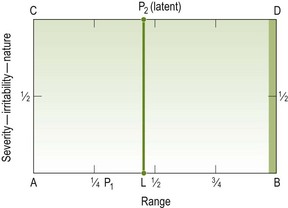
L (3 of 3) qualify
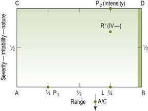
Having decided to stop the movement at L because of the pain's ‘maximum “quality or intensity” ‘ and therefore drawn in point P2 on the line CD, it becomes necessary to qualify what P2 represents: if it is the intensity of the pain that is the reason for stopping at L, then P2 should be qualified thus: ‘P2 (intensity)’.
If, however, the examiner believes that there may be some latent reaction if the joint is moved further even though the pain is not severe, then P2 should be qualified thus: ‘P2 (latent)’ (Fig. A1.12).
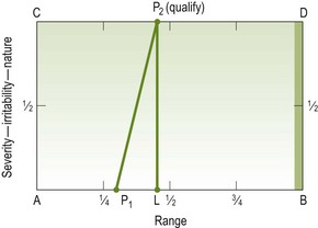
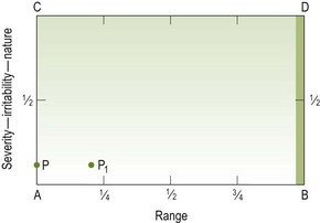
P1P2
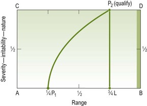
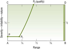
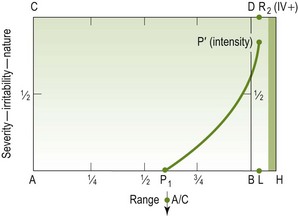
The next step is to depict the behaviour of the pain during the movement between P1 and P2. If pain increases evenly with movement into the painful range, the line joining P1 and P2 is a straight line (Fig. A1.13). However, pain may not increase evenly in this way. Its build-up may be irregular, calling for a graph that is curved or angular. Pain may be first felt at about quarter range and may initially change quickly, and then the movement can be taken further until a limit at three-quarter range is reached (Fig. A1.14).
In another example, pain may be first felt at quarter range and remain at a low level until it suddenly changes, reaching P2 at three-quarter range (Fig. A1.15).
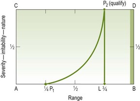
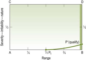
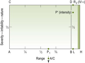
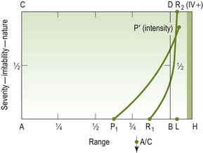
The examples given demonstrate pain that prevents a full range of movement of the joint, but there are instances where pain may never reach a limiting intensity. Figure A1.15 is an example where a little pain may be felt at half range but the pain scarcely changes beyond this point in the range and the end of normal range may be reached without provoking anything approaching a limit to full range of movement. There is thus no point L, and P′ (P′ means P prime) appears on the vertical line BD to indicate the relative significance of the pain at that point (Fig. A1.16). The mathematical use of ‘prime’ in this context is that it represents ‘a numerical value which has itself and unity as its only factors’ (Concise Oxford Dictionary).
If we now return to an example where the joint is painful at rest, mentioned above, an estimate must be made of the amount or quality of pain present at rest, and this appears as P on the vertical axis AC (Fig. A1.17). Movement is then begun slowly and carefully until the original level of pain begins to increase (P1 in Fig. A1.18). The behaviour of pain beyond this point is plotted in the manner already described, and an example of such a graph is given in Figure A1.19. When the joint is painful at rest the symptoms are easily exacerbated by poor handling. However, if examination is carried out with care and skill, no difficulty is encountered.
Again it must be emphasized that this evaluation of pain is purely subjective. Nevertheless, it presents an invaluable method whereby students can learn to perceive different behaviours of pain, and their appreciation of these variations of pain patterns will mature as this type of assessment is practised from patient to patient and checked against the judgment of a more experienced physiotherapist.
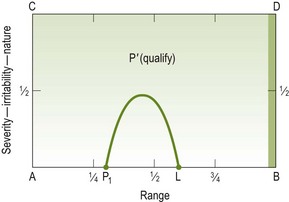
An arc of pain provoked on passive movement might be depicted as shown in Figure A1.20.
Resistance (free of muscle spasm/motor responses)
These resistances may be due to adaptive shortening of muscles or capsules, scar tissue, arthritic joint changes and many other non-muscle-spasm situations.
A normal joint, when completely relaxed and moved passively, has the feel of being well oiled and friction free (Maitland 1980). It can be likened to wet soap sliding on wet glass. It is important for the physiotherapist using passive movement as a form of treatment to appreciate the difference between a free-running, friction-free movement and one that, although being full range, has minor resistance within the range of movement. A strong recommendation is made for therapists to feel the movements suggested in the article.
When depicting a compliance diagram of the forces applied to stretching a ligament from start to breaking point, the graph includes a ‘toe region’, a ‘linear region’ and a ‘plastic region’; the plastic region ends at the ‘break point’ (Fig. A1.21).
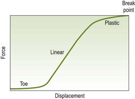
When a physiotherapist assesses abnormal resistance present in a joint movement, physical laws state that there must be a degree of resistance at the immediate moment that movement commences. The resistance is in the opposite direction to the direction of movement being assessed, and it may be so minimal as to be imperceptible to the physiotherapist. This is the ‘toe region’ of the compliance diagram, and it is omitted from the movement diagram as used by the manipulative physiotherapist.
The section of the compliance graph that forms the movement diagram represents the clinical findings of the behaviour of resistance when examining a patient's movement in the linear region only (Fig. A1.22).
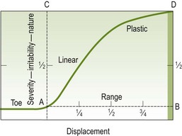
Figure A1.22 Movement diagram (ABCD) within compliance diagram. The dotted rectangular area (ABCD) is that part of the compliance diagram that is the basis of the movement diagram used for representing abnormal resistance (R1R2 or R1R′).
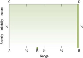
R1
When assessing for resistance, the best way to appreciate the free running of a joint is to support and hold around the joint with one hand while the other hand produces an oscillatory movement back and forth through a chosen path of range. If this movement is felt to be friction free then the oscillatory movement can be moved more deeply into the range. In this way the total available range can be assessed. With experience, by comparing two patients, and also comparing a patient's right side with the left side, the physiotherapist will quickly learn to appreciate minor resistance to movement. Point R1 is then established and marked on the baseline AB (Fig. A1.23).
L – where, L – what
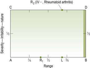
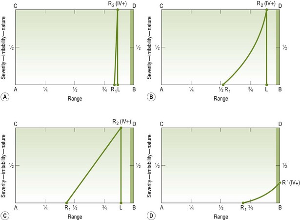
The joint movement is then taken to the limit of the range. If resistance limits movement, the range is assessed and marked by L on the baseline. Vertically above L, R2 is drawn on CD to indicate that it is resistance that limited the range. R2 does not necessarily mean that the physiotherapist is too weak to push any harder; it represents the strength of the resistance beyond which the physiotherapist is not prepared to push. There may be factors such as rheumatoid arthritis which will limit the strength represented by R2 to being moderately gentle. Therefore as with P2, R2 needs to be qualified. The qualification needs to be of two kinds if it is gentle (e.g. R2 (IV−, RA)), the first indicating its strength and the second indicating the reason why the movement is stopped even though the strength is weak (Fig. A1.24). When R2 is a strong resistance (e.g. R2 (IV++)), its strength only needs to be indicated (Fig. A1.24).
R1R2
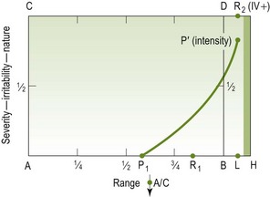
The next step is to determine the behaviour of the resistance between R1 and L, i.e. between R1 and R2. The behaviour of resistance between R1 and R2 is assessed by movements back and forth in the range between R1 and L, and the line depicting the behaviour of the resistance is drawn on the diagram (Fig. A1.25). As with pain, resistance can vary in its behaviour, and examples are shown in Figure A1.25.
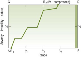
The foregoing resistances have been related to extra-articular structures. However, if the joint is held in such a way as to compress the surfaces, intra-articular resistance might be depicted as in Figure A1.26.
Muscle spasm/motor responses
There are only two kinds of muscle spasm/motor responses that will be considered here: one that always limits range and occupies a small part of it, and the other that occurs as a quick contraction to prevent a painful movement.
Whether it is a spasm or stiffness that is the limiting factor, the range can frequently only be accurately assessed by:
Muscle spasm shows a power of active recoil. In contrast, resistance that is free of muscle activity does not have this quality; rather it is constant in strength at any given point in the range.
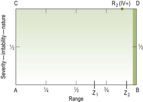
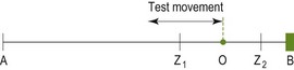
The following examples may help to clarify the point. If a resistance to passive movement is felt between Z1 and Z2 on the baseline AB of the movement diagram (Fig. A1.27), and if this resistance is ‘resistance free of muscle spasm’, then at point ‘O’, between Z1 and Z2 (Fig. A1.28), the strength of resistance will be exactly the same irrespective of how quickly or slowly a movement is oscillated up to it. Furthermore, any increase in strength will be directly proportional to the depth in range, regardless of the speed with which the movement is carried out, i.e. the resistance felt at one point in the movement will always be less than that felt at a point deeper in the range. However, if the block is a muscle spasm and test movements are taken up to a point ‘O’ at different speeds, the strength of the resistance will be greater, with increases in speed.
The first of the two kinds of muscle spasm will feel like spring steel and will push back against the testing movement, particularly if the test movement is varied in speed and in position in the range.
S1
Testing this kind of spasm is done by moving the joint slowly to the point at which the spasm is first elicited, and at this point it is noted on the baseline as S. Further movement is then attempted. If maximum intensity is reached before the end of range, spasm thus becomes a limiting factor.
L – where, L – what
This limit is noted by L on the baseline and S2 is marked vertically above on the line CD. As with P2 and R2, S2 needs to be qualified in terms of strength and quality, for example S2 (IV–, very sharp).
S1S2
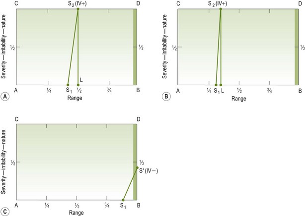
The graph for the behaviour of spasm is plotted between S1and S2 (Fig. A1.29). When muscle spasm limits range it always reaches its maximum quickly, and thus occupies only a small part of the range. Therefore, it will always be depicted as a near-vertical line (Fig. A1.29A,B). In some cases when the joint disorder is less severe, a little spasm that increases slightly but never prohibits full movement may be felt just before the end of the range (Fig. A1.29C).
The second kind of muscle spasm is directly proportional to the severity of the patient's pain: movement of the joint in varying parts of the range causes sharply limiting muscular contractions. This usually occurs when a very painful joint is moved without adequate care and can be completely avoided if the joint is well supported and moved gently. This spasm is reflex in type, coming into action very rapidly during test movement. A very similar kind of muscle contraction can occur as a voluntary action by the patient, indicating a sharp increase in pain. If the physiotherapist varies the speed of the test movements it should be possible to distinguish quickly between the reflex spasm and the voluntary spasm by the speed with which the spasm occurs – reflex spasm occurs more quickly in response to a provoking movement than voluntary spasm. This second kind of spasm, which does not limit a range of movement, can usually be avoided by careful handling during the test.
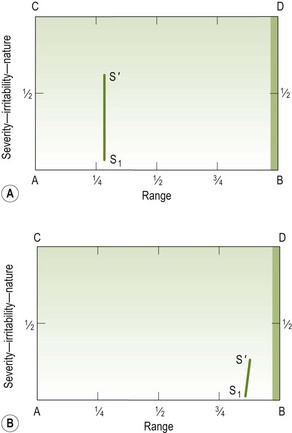
To represent this kind of spasm, a near-vertical line is drawn from above the baseline; its height and position on the baseline will signify whether the spasm is easy to provoke and will also give some indication of its strength. Two examples are drawn of the extremes that may be found (Fig. A1.30A, B).
Modification
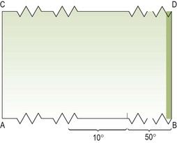
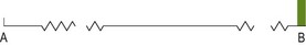
There is a modification of the baseline AB which can be used when the significant range to be depicted occupies only, say, 10° yet it is 50° short of B. The movement diagram would be as shown in Figure A1.31 and, when used to depict a movement, the range between ‘L’ and ‘B’ must be stated.
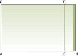
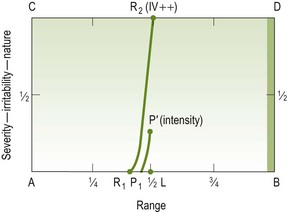
The baseline AB for the hypermobile joint movement to be depicted would be the same as that shown earlier where grades of movement are discussed, and the frame of the movement diagram would be as in Figure A1.32.
Having discussed at length the graphing of the separate elements of a movement diagram, it is now necessary to put them together as a whole.
Compiling a movement diagram
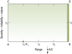
This book places great emphasis on the kinds and behaviours of pain as they present with the different movements of disordered joints. Pain is of major importance to the patient and therefore takes priority in the examination of joint movement. The following demonstrates how the diagram is formulated. When testing the acromioclavicular (A/C) joint by posteroanterior pressure on the clavicle (for example) the routine is as follows.
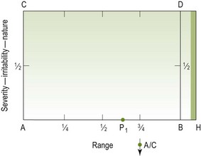
Step 1 P1
Gentle, increasing pressure is applied very slowly to the clavicle in a posteroanterior direction and the patient is asked to report when pain is first felt. This point in the range is noted and the physiotherapist then releases some of the pressure from the clavicle and performs some oscillatory movements, again asking if the patient feels any pain. If pain is not felt, the oscillation should then be carried out slightly deeper into the range. Conversely, if pain is felt, the oscillatory movement should be withdrawn in the range. By these oscillatory movements in different parts of the range, the point at which pain is first felt with movements can be identified and is then recorded on the baseline of the movement diagram as P1 (Fig. A1.33). The estimation of the position in the range of P1 is best achieved by performing the oscillations at what the physiotherapist feels is one-quarter range, then at one-third range and then at half range. By this means, P1 can be very accurately assessed. Therefore the two steps to establishing P1 are:
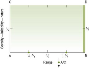
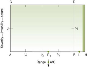
Step 2 L – where
Having found P1 the physiotherapist should continue further into the range with the posteroanterior movements until the limit of the range is reached. The therapist identifies where that position is in relation to the normal range and records it on the baseline as point L (Fig. A1.34).
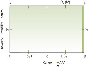
Step 3 L – what
For the hypomobile joint the next step is to decide why the movement was stopped at point L. This means that the joint has been moved as far as the examiner is willing to go but has not made it reach ‘B’. Having decided where ‘L’ is, the examiner has to determine the reason for stopping at L; what it was that prevented the examiner reaching ‘B’. Assume, for the purpose of this example, that it was physical resistance, free of muscle spasm that prevented movement beyond L. Where the vertical line above L meets the horizontal projection CD, it is marked as R2 (Fig. A1.35). The R2 needs to be qualified using words or symbols to indicate what it was about the resistance that prevented the examiner stretching it further; for example the patient may have rheumatoid arthritis and the examiner may not be prepared to go further (see Fig. A1.24) or to push harder than grade IV (Fig. A1.35).
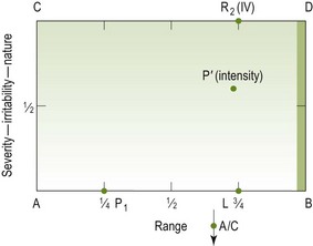
Step 4 P′ and defined
The physiotherapist then decides the quality, nature or the intensity of the pain at the limit of the range. This can be estimated in relation to two values:
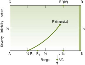
By this means the intensity of the pain is fairly easily decided, thus enabling the physiotherapist to put P′ on the vertical above L in its accurately estimated position (Fig. A1.36).
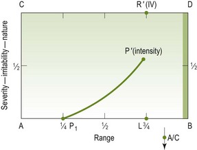
If the limiting factor at L were P2, then Step 4 would be estimating the quality or intensity of R′ and defining it (Fig. A1.37).
Step 5 Behaviour of pain P1P2 or P1P′
The A/C joint is then moved in a posteroanterior direction between P1 and L to determine – by watching the patient's hands and face and also by asking the patient – how the pain behaves between P1 and P2 or between P2 and P′: in fact it is better to think of the pain between P1 and L because at L, pain is going to be represented as P2 or P′. The line representing the behaviour of pain is then drawn on the movement diagram, i.e. the line P1P2 or between P1 and P′ is completed (Fig. A1.38).
Step 6 R1
Having completed the representation of pain, resistance must be considered. This is achieved by receding further back in the range than P1, where, with carefully applied and carefully felt oscillatory movements, the presence or not of any resistance is ascertained. Where it commences is noted and marked on the baseline AB as R1 (Fig. A1.39).
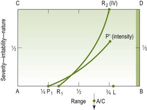
Step 7 Behaviour of resistance R1R2
By moving the joint between R1 and L the behaviour of the resistance can be determined and plotted on the graph between points R1 and R2 (Fig. A1.40).
Step 8 S1S′
If no muscle spasm has been felt during this examination and if the patient's pain is not excessive, the physiotherapist should continue the oscillatory posteroanterior movements, but perform them more sharply and quicker to determine whether any spasm can be provoked. If no spasm can be provoked, then there is nothing to record on the movement diagram. However, if with quick, sharper movements a reflex type of muscle spasm is elicited to protect the movement, this should be drawn on the movement diagram in a manner that will indicate how easy or difficult it is to provoke (i.e. by placing the spasm line towards A if it is easy to provoke, and towards B if it is difficult to provoke). The strength of the spasm provoked is indicated by the height of the spasm line, S1S′ (Fig. A1.41).
Thus the diagram for that movement is compiled showing the behaviour of all elements. It is then possible to access any relationship between the factors found on the examination. The relationships give a distinct guide as to the treatment that should be given, particularly in relation to the ‘grade’ of the treatment movements, i.e. whether ‘pain’ is going to be treated or whether the treatment will be directed at the resistance.
Summary of steps
Compiling a movement diagram may seem complicated, but it is not. It is a very important part of training in manipulative physiotherapy because it forces the physiotherapist to understand clearly what is felt when moving the joint passively. Committing those thoughts to paper thwarts any guesswork, or any ‘hit-and-miss’ approach to treatment. Table A1.1 summarizes the steps taken in compiling a movement diagram where resistance limits movement, and the steps taken where pain limits movement.
Table A1.1
Steps taken in compiling a movement diagram
| Where resistance limits movement | Where pain limits movement |
| 1. P1 (a) slow | 1. P1 (a) slow |
| (b) oscillatory | (b) oscillatory |
| 2. L – where | 2. L – where |
| 3. L – what (and define) R2 | 3. L – what (and define) P2 |
| 4. P′ (define) | 4. P1 P2 (behaviour) |
| 5. P1 P′ (behaviour) | 5. R1 |
| 6. R1 | 6. R′ (define) |
| 7. R1 R2 (behaviour) | 7. R1 R′ (behaviour) |
| 8. S (defined) | 8. S (defined) |
Modified diagram baseline
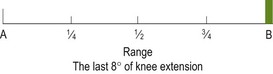
When either the limit of available range is very restricted (i.e. L is a long way from B), or when the elements of the movement diagram occupy only a very small percentage of the full range, the basis of the movement diagram needs modification. This is achieved by breaking the baseline as in Figure A1.42. The centre section can then be identified to represent any length, in any part of the minimal full range. When the examination findings are only to be elicited in the last, say, 8° of a full range, point A in the range is changed and the line AB is suitably identified as in Figure A1.43. This example demonstrates that from A to B is 8°, and A to one-quarter is 2°, and so on.
Example – range limited by 50%
Marked stiffness, with ‘L’ a large distance before ‘B’, necessitates a modified format of the movement diagram. The example will be restricted knee flexion, a longstanding condition following a fracture.
The first element is R1 and the distance between R1 and L is only 12°. Pain is provoked only by stretching (Fig. A1.44). If the movement diagram were drawn on an unmodified format it would be as in Figure A1.45. Figure A1.45 clearly wastes considerable diagram space and is difficult to interpret. With the same joint movement findings represented on the modified format of the movement diagram it becomes clearer and much more useful. The modified format of the baseline of the diagram (Fig. A1.44) requires only two extra measurements to be stated:
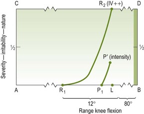
Knowing that R1 to L equals 12° makes it easy to see that R1 is approximately 7° before P1. Because of the increased space allowed to represent the elements of the movement, the behaviour is also far easier to demonstrate.
Clinical example – hypermobility
This example is included for the express purpose of clarifying the misconceptions that exist about hypermobility and the direct influence that some authors and practitioners afford it in restricting passive movement treatment.
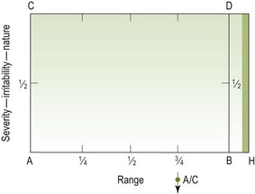
If the movement (using the same acromioclavicular joint being tested with posteroanterior movements), before having become painful, were hypermobile, the basic format of the movement diagram would be shown as in Figure A1.46.
If it becomes painful and requires treatment the movement diagram could be as follows.
Step 3 L – what (and define)
The method is the same as in Example 1; see also Figure A1.49.
Step 4. P′ define (Fig. A1.50)
Step 5. P1P′ behaviour (Fig. A1.51)
Step 6. R1 (Fig. A1.52)
Step 7. R1R2 behaviour (Fig. A1.53)
Treatment
Hypermobility is not a contraindication to manipulation. Most patients with hypermobile joints, one of which becomes painful, have a hypomobile situation at that joint. They are therefore treated on the same basis as is used for hypomobility. It makes no difference whether the limit (L) of the range, on examination, is found to be beyond the end of the average-normal range (as in the example above, L being beyond B) or before it (L being on the side of B). Proof of hypomobility is validated by assessment at the end of successful treatment.
References
Chesworth, BM, MacDermid, JC, Roth, JH, et al. Movement diagram and ‘end-feel’ reliability when measuring passive lateral rotation of the shoulder in patients with shoulder pathology. Phys Ther. 1998;78:593–601.
Latimer, J, Lee, M, Adams, R. The effects of training with feedback on physiotherapy students’ ability to judge lumbar stiffness. Man Ther. 1996;1:266–270.
Lee, R, Evans, J. Towards a better understanding of spinal posteroanterior mobilization. Physiotherapy. 1994;80:68–73.
Maitland, GD. The hypothesis of adding compression when examining and treating synovial joints. J Orthop Sports Phys Ther. 1980;2:7–14.
Maitland, GD. Peripheral Manipulation, ed 3. Oxford: Butterworth-Heinemann; 1991.
Maitland, GD. Neuro/musculoskeletal Examination and Recording Guide, ed 5. Adelaide: Lauderdale Press; 1992.
Petty, N, Maher, C, Latimer, J, et al. Manual examination of accessory movements-seeking R1. Man Ther. 2002;7:39–43.
Snow, CP. Strangers and Brothers. London: Penguin Books; 1965.