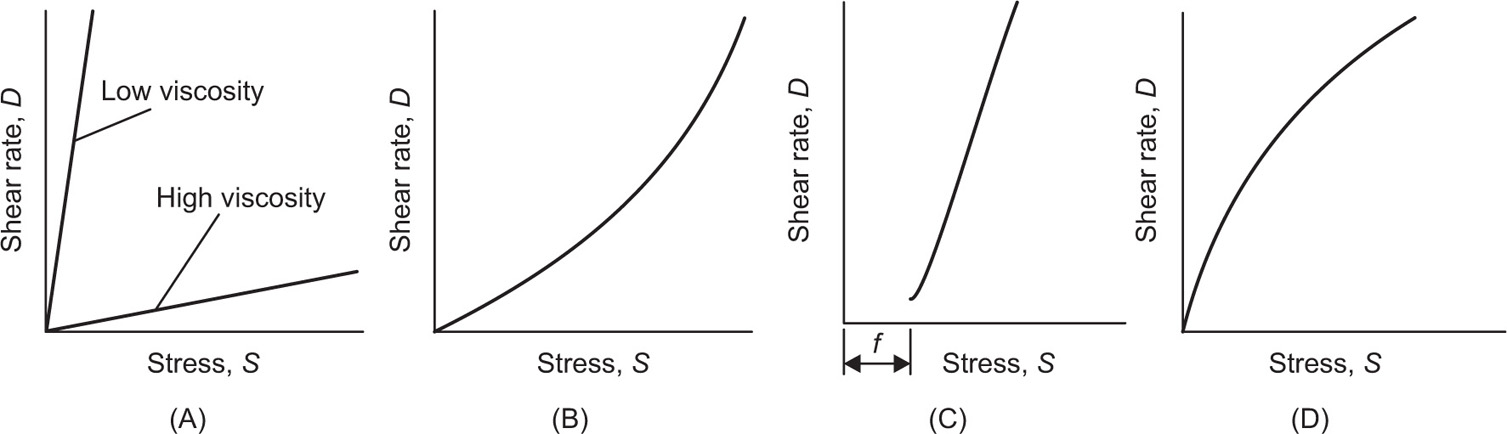
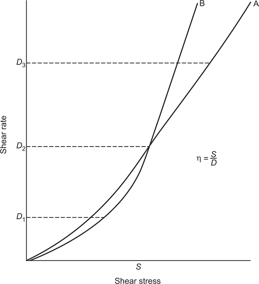
The viscosity of a Newtonian liquid is completely defined by a single figure, the coefficient of viscosity. This coefficient is the ratio of shearing stress rate of shear and provided that streamline flow is maintained, it is of course independent of the actual rate of shear. Many colloidal dispersions, suspen- sions and emulsions cannot be characterized by a viscosity coefficient and it is necessary to determine the relationship between stress and rate of shear over a wide range of shear rate. The resulting plot of stress versus rate of shear is known as a flow curve and examples are shown in
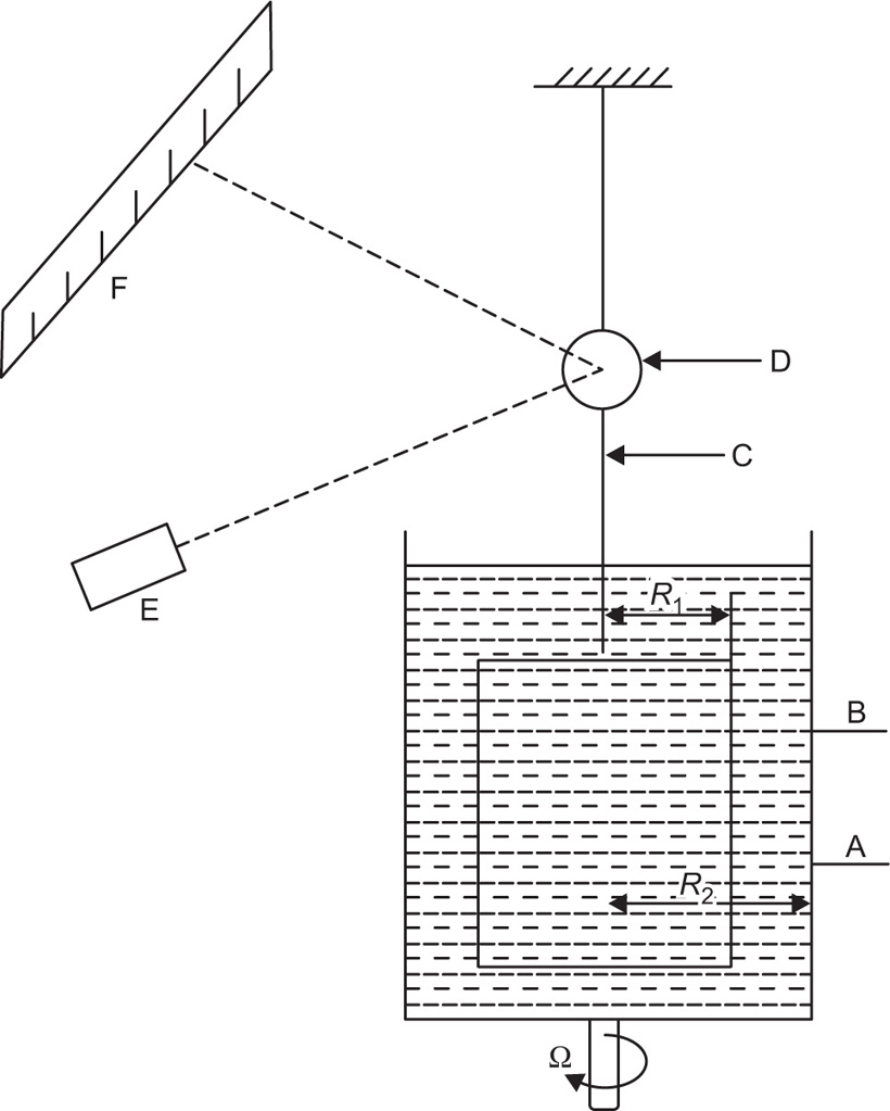
Fig. 10.12. Viscometers that are suitable for these determinations are the coaxial and cone-plate viscometers in which the rate of shear can be varied.
Fig. 10.12A shows the flow curves for two Newtonian liquids of different viscosities.
Pseudoplastic Flow
Solutions of many polymeric substances, e.g. cellulose ethers, tragacanth, alginates, etc. do not show a direct relationship between stress and shear rate (
Fig. 10.12B). At low shear rates the ratio of stress –shear rate (i.e. apparent viscosity) is higher than at the greater shear rates. The flow curve is seen to straighten out at high rates of shear so that the solution reaches a limiting viscosity: This effect is ascribed to molecular interactions resulting in a three-dimensional network structure of solute molecules. For flow to occur this structure must be broken down, and as the rate of shear is increased the molecules will tend to become orientated in the streamlines of the liquid and offer less resistance to flow. Many attempts have been made by rheologists to represent the pseudoplastic curve by equations that have a theoretical basis, but with only limited success. The empirical power law

has been found to represent the flow curve of some pseudoplastic materials. D is the rate of shear and S the shearing stress. The exponent is indicative of non-Newtonian flow. If N has a value of unity the equation reduces to the simple Newtonian equation of flow. The greater the values of N above unity the greater the pseudoplastic behaviour of the material is a constant characteristic of the solution and does not have the same physical significance as a coefficient of viscosity. The equation may be written in logarithmic form:

The plot of log
S against log
D will give a straight line of slope
N and intercept of log
η′ on the log
S axis. The advantages of obtaining an equation to fit a flow curve is that the curve may be more conveniently expressed in terms of the parameters
N and
η′ and this simplifies the compilation of data. For instance, these parameters could be obtained for different concentrations of a polymer in solution, and if a correlation between log
η′ and concentration could be established, the flow properties of a solution of any other concentration could then be calculated.
Kabre et al. (1964) applied this approach to the characterization of the viscosity of a number of natural and synthetic gums.
Plastic Flow
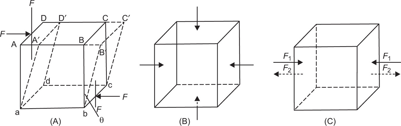
Whereas a Newtonian or pseudoplastic liquid will yield under the application of the smallest shearing force, a plastic material fails to flow until a certain shearing stress has been applied. This is typical of concentrated suspensions of solids, ointments and gels and is thought to result from the aggregation of particles forming a continuous but not orientated, structure throughout the mass. Flow cannot take place until the applied stress exceeds the force of flocculation which causes the particles to adhere together. When flow is initiated the particle layers move relative to the adjacent layers, and the particle contacts are broken but reform again on removal of the stress. Thus the internal structure of the substance is not permanently altered. This behaviour is expressed in
Fig. 10.12C. Flow does not commence until the stress reaches the yield value
f (dynes/cm
2) above which point the shear rate becomes directly proportional to the shear stress and the reciprocal of the slope of graph gives the plastic viscosity
U in poises.
This is expressed by the equation first given by Bingham:

A plastic curve obtained from a coaxial cylinder viscometer is nonlinear over the lower portion of the curve and the yield value f is usually obtained by extrapolation.
Thixotropy
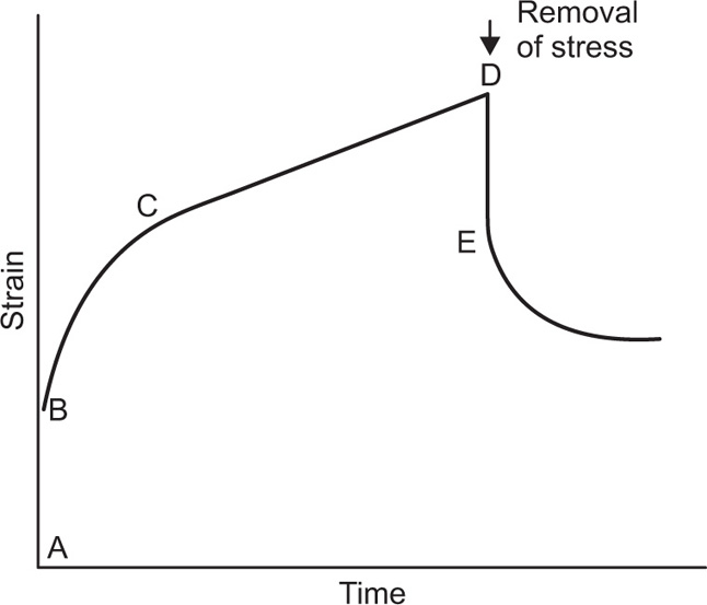
In the description of the different types of non-Newtonian behaviour, it was implied that the viscosity of a fluid might vary with shear rate; it was independent of the length of time that the shear rate was applied, and at the same shear rate would always produce the same viscosity. Most non-Newtonian materials, e.g. particles or macromolecules are colloidal in nature; they may not immediately adapt to the new shearing conditions. Therefore, when such a material is subjected to a particular shear rate, shear stress and consequently viscosity will decrease with time. Furthermore, once the shear stress has been removed, even if the structure that has been broken down is reversible, it may not instantly return to its original structure (rheological ground state). Because of this reason, a characteristic ‘hysteresis loop’ is formed, which shows that a breakdown in the structure has occurred after applying the shearing stress, and the area within the loop may be used as an index of the degree of breakdown. This phenomenon, i.e. breaking and rebuilding of the structure after applying and consequently withdrawing the shear stress, is termed thixotropy.
Thixotropy is defined as a reversible isothermal transition from gel to sol. The word comes from Greek words
thixis (from
thinganein, which means ‘to touch’) and
tropy (from
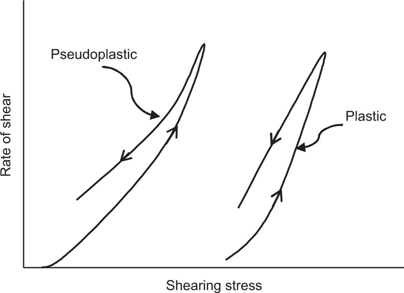
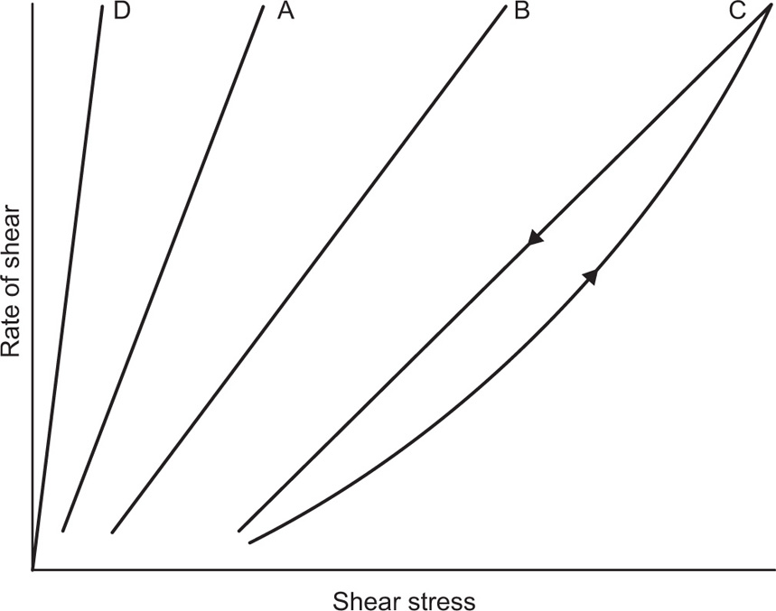
tropos, which means ‘of turning’, ‘changeable’, ‘to turn’, or in simple word ‘to change by touch’). Thixotropy may only be applied to shear thinning system, i.e. plastic and pseudoplastic system. In the case of plastic and pseudoplastic materials, the down curve will be displaced to the right of the up curve, while in case of Newtonian system, the resultant curve is identical with and superimposed on the up curve and
Fig. 10.13 illustrates the flow diagrams of such systems.
It is believed that thixotropic systems are usually composed of asymmetric particles or macromolecules, which are capable of interacting by numerous secondary bonds to produce a loose three-dimensional structure, and confer some degree of rigidity on the system, which resembles a gel. The energy imparted during shearing disrupts these bonds, which causes the interparticle links to be broken; the network therefore disintegrates and the viscosity falls, and a gel–sol transformation occurs. When the shear stress is eventually removed, the structure will tend to reform, although the process is not immediate and will increase with time as the molecules return to the original state under the influence of Brownian motion. For such cases, the rheogram depends on the rate at which shear is increased or decreased and the length of time a sample is suggested to any one rate of shear.
It was seen that a thixotropic material is similar to a pseudoplastic material in one manner; it exhibits lower viscosity as shear increases. However, the thixotropic profile differs substantially from the pseudoplastic profile in the manner in which viscosity recovers from the release of shear. Where viscosity in a pseudoplastic material recovers immediately on release of shear, in a thixotropic material there is a measurable delay in the recovery of viscosity. This delay allows for a period of flow and levelling or film consolidation to occur. Such a delay also allows the graphing of a hysteresis loop in which the viscosity is plotted as a function of both as shear is applied and released. This hysteresis loop allows to display number of properties that are of a system’s rheology, which includes the degree of thixotropy, the absolute viscosity values at a given shear rate, and the speed of viscosity recovery.
Applications of Thixotropy
Thixotropy is a desirable property in liquid pharmaceutical system; ideally it should have a high consistency in the container yet pour or spread easily. If emulsion or suspension, it implies low viscosity, which causes either rapid settling of solid particles in suspension or rapid creaming of emulsion. As we know, according to Stock’s equation (
Eq. 10.9) the rate of sedimentation is proportional to viscosity. Frequent settling of solid produces sediment difficult to redisperse, whereas creaming is the first step towards coalescence. Addition of thixotropic agents, i.e. bentonite magma, clay, colloidal silicon dioxide, microcrystallin cellulose, etc. into suspension or emulsion provides a high viscosity. High viscosity retards sedimentation or creaming as well as flow below the yield stress. When other applicant is desired to pour some of the suspension or emulsion from container, it is shaken well at sufficient shear stress, which breaks the thixotropic structure and lowers the apparent viscosity. Back on shelf the viscosity again slowly increases again and the structure is rebuilt because of the Brownian motion. A similar pattern is required with lotion, cream, ointment and parenteral suspensions for intramuscular depot therapy.
Concentrated parenteral suspension containing about 40–70% w/v of procaine penicillin G in water has a high inherent thixotropy. Breakdown of the structure occurred when the suspension was caused to pass through the hypodermic needle. Consequently, rheological structure was rebuilt and a depot of drug formed at the site of injection in the muscles from which drug was slowly released and made available for absorption.
Measurement of Thixotropy
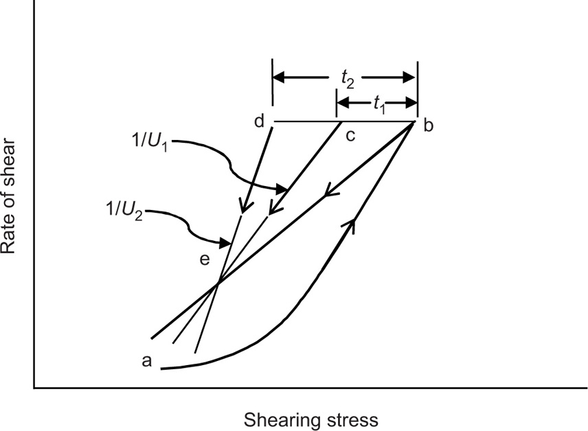
Thixotropy can be quantitatively represented by the area of the hysteresis loop by a coefficient of thixotropic breakdown or by the decay of shearing stress or apparent viscosity as a function of time at constant rate of shear. Structural breakdown or thixotropy can be determined by two approaches. In the first approach, thixotropy is determined by the structural breakdown with time at a constant rate of shear. The shear rate of a thixotropic material is increased in a constant manner from point a to point b and is then decreased at the same rate back to point e. This forms the hysteresis loop abe. If sample was taken to point b and the shear rate held constant for a certain period of time, i.e. for
t1 second, the shearing stress and the consistency would decrease to an extent depending on the time of shear, the rate of shear and the degree of structure in the sample. This would lead to hysteresis loop abce. If the sample has been held at the same rate of shear for
t2 second, this will give abcde loop (
Fig. 10.14). On the basis of such rheogram, a thixotropic coefficient
B, the rate of breakdown with time at constant shear rate, is calculated as:

In which U1 and U2 is plastic viscosity of two down curves obtained after shearing at a constant rate for t1 and t2 sec, respectively. The choice of rate is arbitrary. A more meaningful though time-consuming method for characterizing thixotropic behaviour is to measure the fall in stress with time at several rates of shear.
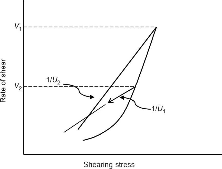
The second approach is to determine the structural breakdown due to increasing shear shown in
Fig. 10.15, in which two hysteresis loops are obtained having different maximum rates of shear,
V1 and
V2. In this case, a thixotropic coefficient
M, the loss in shearing stress per unit increase in shear rate, is obtained from

where U1 and U2 are the plastic viscosities for two separate down curves having maximum shearing rates of V1 and V2, respectively. With this technique, the rates of shears V1and V2 are chosen arbitrarily. The value of M will depend on the rates of shear chosen since these shear rates will affect the down curves and hence the value of U that are calculated.
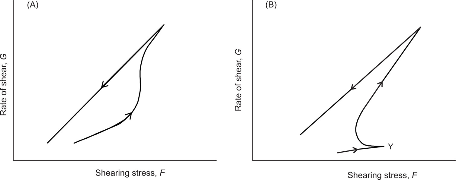
Bulges and Spurs: In some cases different type of thixotropic rheogram is obtained for examples bulges and spurs type rheogram. A concentrated aqueous bentonite gel (10–15% by weight) produces a characteristic bulge in the up curve of a hysteresis loop. This is due to the presence of crystalline plates in a pattern of ‘house-of-cards’ structure, which causes the swelling of the bentonite magmas (
Fig. 10.16A). In another case—procaine penicillin gel formulation for IM injections, the hysteresis loop is in the form of spur-like protrusion. The structure showed a high-yield value,
Y, which traces out a bowed up curve due to sharp breakdown of three-dimensional structure at slow shear rate, as shown in
Fig. 10.16B. It was found that penicillin gels having definite
Y values were very thixotropic, forming intramuscular depots on injection that afforded prolonged blood level of the drug.
Negative Thixotropy: Negative thixotropy, also known as
antithixotropy. It is a rheological phenomenon that represents an increase rather than a decrease in consistency on the down curve. This increase in thickness or resistance to flow with increased tie of shear was observed by
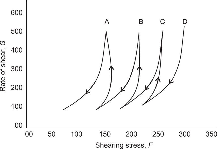
Chong et al. (1960). This effect can be observed in a wide range of polymers and solvents. In case of negative thixotropy, e.g. when magnesium magma was treated alternatively with increasing and decreasing rates of shear,
the magma continuously thickened and then finally reached an equilibrium state in which further cycles of increasing and decreasing shear rates no longer increased the consistency of the magma (
Fig 10.17). The equilibrium system was found to be gel like and providing great suspendability, yet it was readily pourable. In this case the equilibrium state is the sol.
The origin of negative thixotropy is the tendency of a polymer to aggregate in a solvent, giving rise to temporary link aggregates or crystallites or, in other words, it results from an increased collision frequency of dispersed particles or polymer molecules in suspension, which increased interparticle bonding with time. This tendency to aggregate is usually considered to vary along the polymer chain and it is also a change of the small to large number of big particle or floccules, while at rest large floccules break and gain their original structure.
Phenomenon of negative thixotropy is quite different from the dilatant flow in a manner as dilatant systems are deflocculated and contain more than 50% by volume of solid dispersed phase, whereas antithixotropy systems consist of 1–10% solid contents and are flocculated.


 (10.1)
 (10.2)
 (10.3)
 (10.4)
 (10.5)
 (10.6)
 (10.7)
 (10.8)
 (10.9)