Image Quality
In general, the image quality of a computed tomography (CT) scanner can be described by several key performance parameters: high-contrast spatial resolution, low-contrast resolution, temporal resolution, CT number uniformity and accuracy, noise, and artifacts. These parameters are influenced not only by the CT system performance but also by the operator’s selection of protocols such as x-ray tube voltage (in kilovolts [kV]), tube current (in milliamperes [mA]), slice thickness, helical pitch, reconstruction parameters, and scan speed. As often is the case of a real-life problem, tradeoffs have to be made between image quality, dose to the patient, system limitations, patient conditions, and clinical indications. Over the years, many studies have been conducted to understand such tradeoffs (Barnes and Lakshminarayan, 1981; Blumenfeld and Glover, 1981; Hanson, 1981; Hsieh, 2003; Kalender and Polacin, 1995; McCollough and Zink, 2000; Morgan, 1983; Pfeiler et al, 1976; Robb and Mortin, 1991). Clearly, tradeoff decisions between various performance parameters are not as straightforward as would be hoped. Although the design of CT scanners has been evolved significantly over the years to minimize the complexity of parameter selection, even state-of-the-art scanners still depend, in various degrees, on the experience of the operator to produce optimal image quality.
Given the limited scope of this chapter, it is impossible to discuss all factors that affect the image quality of a CT scanner, let alone the tradeoffs among these factors. Instead, only the most important performance parameters are the focus, and, whenever possible, some of the common factors that influence the CT performance and phantoms used to perform quantitative measurements are briefly discussed. Because of the wide availability of the helical/spiral and multislice/volumetric CT scanners in recent years, their specific characteristics and requirements are incorporated into the discussion of each topic, rather than being isolated in a separate section.
HIGH-CONTRAST SPATIAL RESOLUTION
High-contrast spatial resolution of a CT scanner describes the scanner’s ability to resolve closely placed objects that are significantly different from their background. Historically, spatial resolution was defined and measured predominately within the scanning plane. With the popularity of the multislice/volumetric helical CT, however, the cross-plane resolution becomes just as important.
In-Plane Spatial Resolution
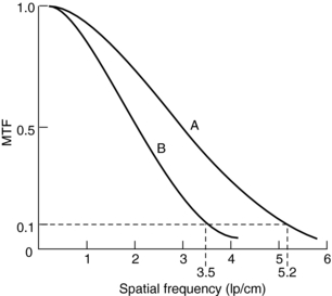
Definition and Measurements: The in-plane resolution is specified in terms of line pairs per centimeter (lp/cm) or line pairs per millimeter (lp/mm). A line pair is a pair of equal-sized black-white bars. Therefore, a bar pattern representing 10 lp/cm is a set of uniformly spaced combshaped bars with 0.5-mm wide teeth. Because the CT acquisition and reconstruction process is band limited (high-frequency contents are suppressed or eliminated), the reconstructed image of a bar pattern is a blurred version of the original object, as illustrated in Figure 9-1. The edges of the bars are softened, and the magnitude of the bar pattern is reduced. If the peak-to-valley magnitude of the original object is normalized as unity, the reconstructed peak-to-valley is smaller. For example, in Figure 9-1, at 1 lp/cm spatial frequency, the reconstructed peak-to-valley magnitude is 0.88; at 2 lp/cm, the magnitude is 0.59, and so on. In general, the magnitude reduces as the frequency (lp/cm) of the bar pattern increases. If the spatial frequency is plotted as a function of the image fidelity, a smooth curve is obtained (Fig. 9-2). This is often referred to as the modulation transfer function (MTF) of the system. MTF can be used to compare the performance of different CT systems. For example, scanner A can image 5.2 lp/cm at 0.1 MTF compared with scanner B, which can only image 3.5 lp/cm at 0.1 MTF (Fig. 9-3). This simply means that scanner A has a better spatial resolution capability than scanner B.
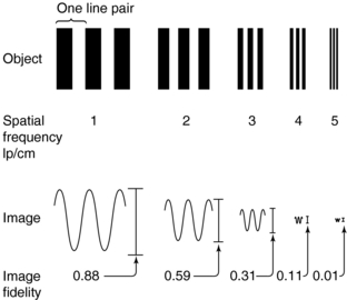
FIGURE 9-1 A bar pattern (object) consists of line pairs (lp, one line pair equals one bar plus one space). The number of line pairs per unit length is called the spatial frequency. Large objects have a low spatial frequency, whereas small objects have a high spatial frequency.
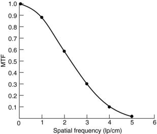
FIGURE 9-2 A modulation transfer function (MTF) curve obtained from the data given in Figure 9-1.
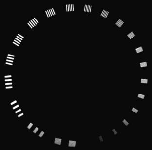
An ideal system would have a flat MTF curve, a unity response independent of frequency. Such a system ensures that the object can be reproduced exactly. For practical systems, however, the frequency response falls off quickly as the frequency increases. Three points on the MTF curve are of particular interest: 50%, 10%, and 0%. The 50% MTF refers to the frequency at which the magnitude of the MTF curve drops to 50% of its peak value. Similarly, the 10% and 0% MTF refer to the frequencies at which the MTF drops to 10% and 0% of the peak value. Various phantoms have been designed specifically to measure the MTF of the system. For example, the Catphan High Resolution Insert contains high-density metal bar patterns ranging from 1 to 21 lp/cm, as shown in Figure 9-4.
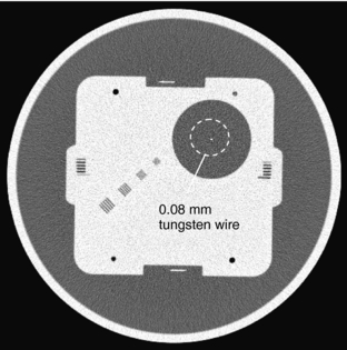
Alternatively, the MTF of a system can be derived from the point spread function (PSF) of the system (Hsieh, 2003). PSF is defined as the system response to a Dirac delta function. If the scanned object is a high-density thin wire placed perpendicular to the scanning plane, and as long as the diameter of the wire is significantly smaller than the resolution of the system, the wire can be considered as a Dirac delta function. The reconstructed image of such wire is then simply the PSF of the system. By definition, MTF is related to PSF by the magnitude of the Fourier transform. As an illustration, Figure 9-5 depicts a GE Performance Phantom with a 0.08-mm diameter tungsten wire submerged in water. If we isolate the wire portion of the image and remove its background (Fig. 9-6, A) and take the Fourier transform of this image (Fig. 9-6, B), the MTF of the CT system can be obtained by averaging the frequency domain image over 360 degrees, as shown by the curve in Figure 9-6.

Factors Affecting Resolution: Many factors affect the in-plane spatial resolution. The most dominating factors are the x-ray focal spot size and shape, detector cell size, scanner geometry, and sampling frequency. Although these factors are largely determined by CT manufacturers, operators do have limited control. For example, most CT scanners have more than one x-ray focal spot to account for an increased tube loading. By properly selecting the x-ray tube current, an operator has the option to use either the small spot (lower tube current, higher spatial resolution) or the large spot (higher tube current, lower spatial resolution).
The in-plane resolution is also strongly influenced by the reconstruction algorithm. Chapter 6 indicates that image reconstruction involves two mathematical procedures: convolution and back-projection. Essentially, if the projection profiles are back-projected without correction, blurring results (Fig. 9-7, A). To sharpen the image, a convolution process (a ramp filter) is applied to modify the frequency contents of the projection before back-projection (Fig. 9-7, B). The convolution algorithm, or kernel, affects the appearance of image structures. Convolution algorithms have been developed for each anatomic-specific application. In general, these algorithms are applied to emphasize soft tissue (standard algorithm) and bone (bone algorithm). The former is applied to the mid brain, pancreas, adrenal, or any soft tissue region, and the latter is applied to bony structures such as the inner ear and extremities. As an illustration, two images in Figure 9-8 are reconstructed from the same scan data with two different reconstruction kernels. Figure 9-8, A, was reconstructed with a standard kernel and Figure 9-8, B, with a bone kernel. It is clear that the bone kernel produces a much sharper image (higher spatial resolution) as demonstrated by the bar patterns. It is also worth pointing out that increased noise often accompanies the spatial resolution improvement. Similar clinical examples are given in Figure 9-9, where a lung scan was reconstructed with a standard (A) and a lung kernel (B).
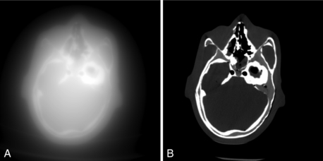
FIGURE 9-7 Images of a head phantom to illustrate the impact of the convolution process. A, Reconstructed with back-projection only. B, Reconstructed with filtered back-projection.
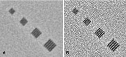
FIGURE 9-8 Impact of the selection of reconstruction kernel on spatial resolution. A, Reconstructed with a standard kernel. B, Reconstructed with a bone kernel.
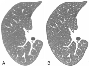
FIGURE 9-9 A patient chest scan reconstructed with different kernels. A, Standard algorithm. B, Lung algorithm.
Another parameter that affects the spatial resolution is the reconstruction field of view (FOV). On the basis of the Nyquist sampling theory, the sampling interval (pixel size) has to be sufficiently small to support the reconstruction and visualization of small objects. The pixel size is related to FOV by the following equation:

For a 50-cm FOV at a matrix size of 512 × 512, the pixel size is 0.98 mm (500 mm/512). If the FOV is reduced to 10 cm, the pixel size is 0.20 mm. (This is often referred to as targeting.) To illustrate the impact of pixel size, Figure 9-10 depicts images reconstructed with the same projection dataset at two different FOVs. Both Figures 9-10, A and B, were reconstructed with a 50-cm FOV. The reconstructed image was then interpolated in image space to a 10-cm FOV to produce Figure 9-10, B. Figure 9-10, C, was reconstructed directly to 10-cm FOV. Note that for the 10-cm target-reconstructed image, all bar patterns are clearly visible, whereas even the fourth largest bar pattern is barely visible for the reconstructed images with 50-cm FOV.
Cross-Plane Spatial Resolution
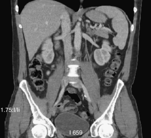
The introduction of helical/spiral and multislice/volumetric CT has fundamentally changed the way many radiologists view CT images. Historically, CT images were always viewed one slice at a time. New technologies have enabled radiologists to view images in three dimensions by using multiplanar reformat (MPR), maximum-intensity-projection (MIP), or volume rendering (VR). One such example is shown in Figure 9-11, where a coronal view of a patient study is displayed. It is difficult to tell from the image alone whether the data were acquired slice by slice or directly in the coronal plane. This demonstrates that the spatial resolution of the state-of-the-art scanner is nearly isotropic.
Improved cross-plane spatial resolution also reduces artifacts caused by partial volume averaging. Figure 9-12 presents a comparison of the spatial resolution afforded by two slices of different thicknesses. Thin slice imaging of lung “is currently the most accurate noninvasive tool for evaluation of lung structure” (Mayo, 1991).

FIGURE 9-12 Comparison of the degree of spatial resolution of slices with two different thicknesses. The spatial resolution of the thinner slice (B) taken with 1.5-mm collimation is apparent when compared with the image of the slice taken with 10-mm collimation (A). From Mayo JR: High-resolution computed tomography, Radiol Clin North Am 29:1043-1048, 1991.
Cross-plane spatial resolution is traditionally described by the slice sensitivity profile (SSP). Similar to the in-plane resolution, SSP represents the system response to a Dirac delta function. In practice, the Dirac delta function is often approximated by an object whose thickness is significantly smaller than the slice thickness of the system. For example, researchers use a small bead or a thin disk to perform SSP measurement. The disk is placed perpendicular to the z-axis and a series of scans are collected to construct the SSP. In many cases, the SSP curve itself is replaced by two numbers: the full width at half-maximum (FWHM) and the full width at tenth-maximum (FWTM). Definitions of FWHM and FWTM are illustrated in Figure 9-13, where FWHM represents the distance between two points on the SSP curve whose intensity is 50% of the peak and FWTM represents the distance between two points on the SSP whose intensity is 10% of the peak.
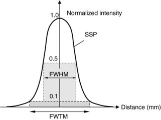
FIGURE 9-13 Illustration of FWHM and FWTM. FWHM represents the distance between two points on the SSP curve whose intensity is 50% of the peak. FWTM represents the distance between two points on the SSP whose intensity is 10% of the peak.
A more convenient method of measuring SSP is to use a shallow-angled slice ramp (Goodenough et al, 1977; Hsieh, 2001). A line or thin strip is placed at a shallow angle with respect to the x-y plane. During the scan, the line or thin strip is projected onto the x-y plane, as shown in Figure 9-14. On the basis of simple trigonometry, the SSP in z is magnified by a factor, 1/tan(θ), where θ is the angle of the strip formed with the x-y plane. When θ is small, the magnification factor is large. For example, Catphan phantom uses a 23-degree ramp to produce a 2.4-fold enlargement in the measured SSP. Therefore, the FWHM of the system, ZFWHM, can be calculated from the FWHM measurement of the wire in the reconstructed image, WFWHM, by:
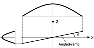
FIGURE 9-14 Illustration of measurement of slice-sensitivity profile by a shallow-angled slice ramp. The slice ramp is projected onto the x-y plane during reconstruction. A magnified version of the SSP is produced.

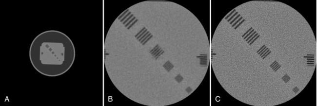
For illustration, Figure 9-15 shows a GE Performance phantom scanned with a 5-mm and a 10-mm detector aperture in a step-and-shoot mode. It is clear from the figure that the image of the slice ramp is twice as wide for the 10-mm case as for the 5-mm, indicating a linear relationship between the width of the reconstructed wire and the thickness of the slice. It is also clear that a significant reduction in contrast is observed for the 10-mm case as a result of the partial volume effect.
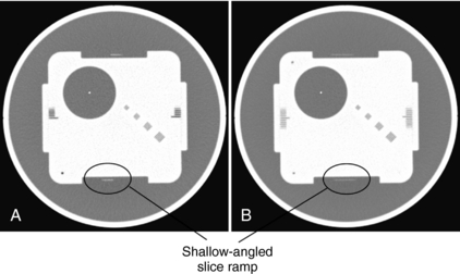
FIGURE 9-15 Illustration of the use of slice ramp to measure SSP. A, Acquired with 5-mm slice thickness in step-and-shoot mode. B, Acquired with 10-mm slice thickness in step-and-shoot mode.
It should be noted that once the SSP is obtained, MTF can be calculated in a straightforward fashion by taking the Fourier transform of the SSP. As the spatial resolutions in all orientations become isotropic, it is more convenient and reasonable to specify both the in-plane and cross-plane resolution in a similar fashion, such as MTF.
LOW-CONTRAST RESOLUTION
One of the key advantages of CT over conventional radiography is its ability to observe low-contrast objects whose density is slightly different from the background. In CT, this is sometimes referred to as the sensitivity of the system (Hounsfield, 1978). To understand low-contrast resolution, consider three tissues of different densities and atomic number (Z), as shown in Figure 9-16. If these tissues were imaged by conventional radiography, the obtained image would have shown good contrast between bone and soft tissue (muscle and fat) only. The values of the density and Z for muscle and fat are too close to be clearly distinguished by radiography, and they appear as “soft tissue shadows.” The contrast between bone with a Z of 13.8 and soft tissue with a Z of 7.4 is apparent because of the significant difference between the densities and Z of these two tissues. CT, on the other hand, can image tissues that vary only slightly in density and atomic number. Although radiography can discriminate a density difference of about 10% (Curry et al, 1990), CT can detect density differences from 0.25% to 0.5%, depending on the scanner (Hsieh, 2003).
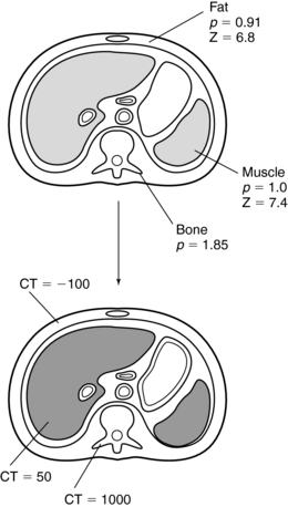
FIGURE 9-16 Densities (p) and atomic numbers (Z) for three types of tissue. When they are imaged by CT, excellent low-contrast resolution is obtained. From Bushong S: Radiologic science for technologists, ed 9, St Louis, 2009, Mosby.
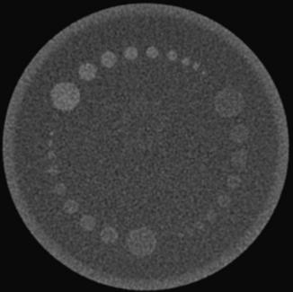
Low-contrast resolution can be measured with phantoms that contain low-contrast objects of different sizes. The low-contrast performance or low-contrast detectability (LCD) of the scanner is typically defined as the smallest object that can be visualized at a given contrast level and dose. For illustration, Figure 9-17 shows a low-contrast portion of a Catphan. There are three sets of discs with contrast of 0.3%, 0.5%, and 1.0%, and the sizes of the discs are 2 mm, 3 mm, 4 mm, 5 mm, 6 mm, 7 mm, 8 mm, 9 mm, and 15 mm. In CT, the contrast level is specified in terms of the percent linear attenuation coefficient. A 1% contrast means that the mean CT number of the object differs from its background by 10 Hounsfield units (HU).
Factors That Affect Low-Contrast Detectability
From the definition of LCD, it can easily be concluded that the visibility of an object depends not only on its size but also on its contrast (intensity difference) to the background. This is easily demonstrated with the Catphan. Note that the three sets of objects are of matching sizes. The discs located from the 10 o’clock to 2 o’clock positions are more easily visualized than the ones that are located from the 2 to 6 o’clock positions. The difference in contrast between these two sets is 7 HU. The figure also illustrates the impact of the object size on the LCD. As the object size decreases, the confidence level of identifying a 0.3% disc decreases.
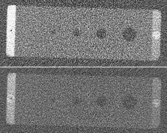
The LCD definition also implies that an object’s visibility is highly influenced by the presence of noise. To demonstrate this effect, the low-contrast portion of a GE Performance Phantom was scanned with two different tube currents: 200 mA and 50 mA; the reconstructed images are shown in Figure 9-18. All other acquisition parameters were kept the same. The noise for the 50-mA scan is a factor of two higher compared with the 200-mA case (one fourth of the dose). For the 200-mA scan, all four low-density holes are clearly identifiable, whereas the smallest hole is obscured by the noise for the 50-mA scan.
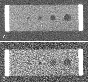
FIGURE 9-18 Illustration of the impact of noise to low-contrast detectability. A, Acquired with 200 mA and standard algorithm. B, Acquired with 50 mA and standard algorithm.
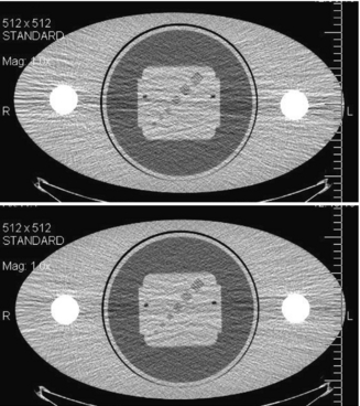
Many factors affect the noise level in the reconstructed images. Some of them can be controlled by the operator, and others are outside the operator’s reach. The parameters under operator control include x-ray tube voltage (in kV), tube current (in mA), scan speed (in seconds), helical pitch, and slice thickness. The selection of the parameters, however, is not straightforward. For example, by increasing the tube current, a noise reduction, better LCD, can be achieved. However, increased tube current translates to a higher dose to the patient and, potentially, runs the risk of a tube cooling (forced delay during scans to prevent the tube from overheating). Similarly, although the use of a higher tube voltage (kV) results in improved x-ray photon statistics (therefore lower noise in the image), the quality of the x-ray beam is somewhat compromised because the visibility of low-contrast objects depends on the presence of low-energy photons, which are disproportionally less for the higher tube voltage. Consequently, LCD may not improve or degrade with an increased kV. The same applies to the selection of slice thickness. Although, in general, an image with a thicker slice contains more x-ray photons (less noise), the partial volume effect can reduce the visibility of smaller objects. This is illustrated in Figure 9-19, where the low-contrast portion of the GE Performance Phantom was reconstructed with 3.75-mm and 7.5-mm slice thickness. Because the phantom is made of a thin plate (less than 1 mm in thickness), a thicker slice produces a larger partial volume effect and reduces the contrast of the object. As a result, although the noise is reduced with the 7.5-mm thickness, the LCD of the low-density objects is reduced as well.
TEMPORAL RESOLUTION
Temporal resolution is an indication of a CT system’s ability to freeze motions of the scanned object. An oversimplified analogy is the “shutter” speed of a camera. When a photo is taken at a sports event, a higher shutter speed should be used to reduce the blurring effects caused by the moving athletes. The awareness and importance of the temporal resolution for CT scanners has increased significantly in recent years thanks to cardiac imaging. Because the heart motion is continuous and often irregular, cardiac imaging is one of the most challenging clinical applications for CT.
Factors That Affect Temporal Resolution
There are several methods that improve a CT scanner’s ability to freeze the cardiac motion. The most straightforward way to reduce or eliminate the motion impact is to increase the scan speed. The state-of-the-art third-generation multislice scanners are capable of rotating at speeds of 0.3 to 0.4 seconds per gantry rotation. Considering the size of a typical CT gantry (1 meter), and the weight of the components on the rotating side (hundreds of pounds), the centrifugal force is huge. One attempt to overcome the mechanical difficulty is the use of an electron-beam scanner in which high-speed electrons are deflected by the specially designed magnetic field so that x-ray photons are generated along an arc surrounding the patient. Because there is no moving part for such a scanner, scan speeds as high as 33 milliseconds can be achieved.
It should be noted that even at the speed of 33 milliseconds, it is insufficient to completely freeze the cardiac motion. Therefore all third-generation CT scanners also rely on reconstruction algorithms that use less than a full rotation of projection data for reconstruction (Parker, 1982). The most commonly used algorithm is the so-called half-scan algorithm in which the projection dataset in the view range of 180 degrees plus fan angle are used. For typical CT scanner geometries, this represents a 220-degree, or roughly 40%, improvement in terms of temporal resolution. To further improve the temporal resolution of the scanner, multisector reconstruction is also used in which the 220 degrees of projection data are acquired over multiple cardiac cycles (Hsieh, 2003). Typically, the dataset is uniformly divided over these heart cycles to optimize the performance. Because of the limited scope of this chapter, the details are not discussed.
Techniques to Reduce Motion Impact
A technique used by all CT vendors incorporates a physiological gating device for cardiac imaging (Hsieh et al, 1999; Kachelriess et al, 2000). Although this approach does not improve the temporal resolution of the scanner, it helps to minimize the heart motion. In a typical cardiac motion cycle, there are quiescent time periods in which the heart is in a relatively motionless state. These correspond to the diastole and systole phases of the heart. Therefore if the data acquisition takes place during these time periods, fewer motion artifacts can be expected. This can be accomplished by synchronizing the data acquisition and reconstruction with an electrocardiographic (ECG) signal, as shown in Figure 9-20. This can be performed either retrospectively or prospectively. The advantage of a prospective gating is the reduction in x-ray dose to the patient. The x-ray tube can be shut off during the non–data acquisition periods to minimize the x-ray exposure. The disadvantage of the prospective gating is its reliance on the regularity of the heart motion because the data acquisition timing for the current cardiac cycle is predicted on the basis of previous heart cycles. For compromise, x-ray tube current modulation is often used in practice in which the x-ray tube current is reduced to a fraction of the peak current during the nonquiescent time periods. It provides a balance between patient dose and image quality. To illustrate the impact of ECG gating, Figure 9-21 depicts two reconstructed cardiac images, with and without the proper ECG gating. Motion artifact reduction with ECG gating is obvious.

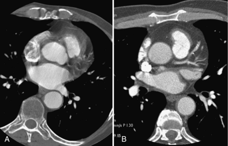
FIGURE 9-21 Impact of ECG gating in cardiac imaging. A, Nongated cardiac acquisition. B, ECG-gated acquisition.
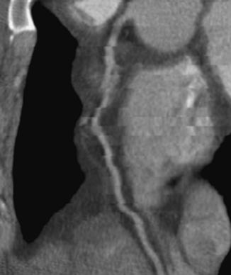
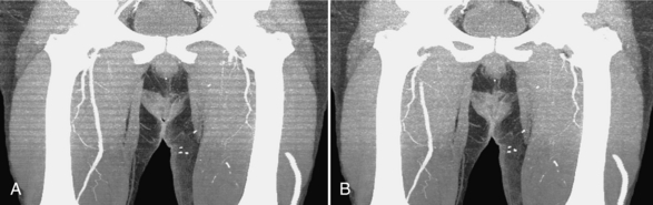
For cardiac imaging, there is another important factor that affects the image quality: coverage. Note that all the commercially available CT scanners today cannot cover the entire heart (12 to 16 cm) in a single rotation. Consequently, the heart volume has to be scanned over multiple heart cycles, with each cycle covering a subsection of the heart. Superb temporal resolution only ensures that within each subsection the motion-induced image degradation is kept to a minimum. It does not guarantee, however, that the heart is in exactly the same state from one subsection to the next. This is determined mainly by the consistency of the heart motion from cycle to cycle. Studies have shown that the probability of a stable heart rate decreases quickly as the total data acquisition time increases. The total data acquisition time is determined by the gantry speed, helical pitch, and detector coverage. For the same gantry speed and helical pitch, a larger detector-coverage translates to a faster study time and, in turn, an improved probability of a consistent cardiac volume. Figure 9-22 shows a reformatted image of a heart vessel with phase misregistration. The vessel looks discontinuous and can lead to misdiagnosis.
CT NUMBER ACCURACY AND UNIFORMITY
The CT number is related to the attenuation coefficient of the object by the following equation:
where μw is the attenuation coefficient of water. On the basis of this definition, two points are defined precisely on the CT number scale. The first is water with a CT number of 0 and the second is air with a CT number of −1000. Because water is similar to the soft tissue in terms of attenuation characteristics, it is important to establish its accuracy for CT scanners. Nearly all CT manufacturers provide phantoms filled with water for such testing. When the phantom is scanned, the average CT number in the water portion should be fairly close to 0.
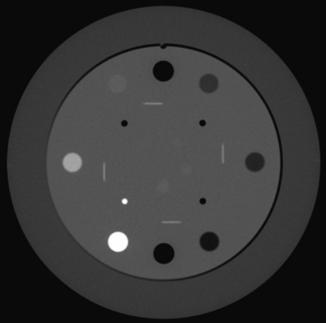
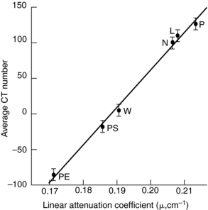
Linearity is another important parameter in CT image quality. Linearity refers to the relationship of CT numbers to the linear attenuation coefficients of the object to be imaged. This can be checked by a daily calibration test, during which an appropriate phantom is scanned to ensure that the CT numbers for water and other known materials of which the phantom is made are correct. Such phantom characteristics are given in Table 9-1. For illustration, Figure 9-23 depicts a linearity section of the Catphan with the large cylinders filled with Teflon, Delrin, acrylic, polystyrene, air, polymethylpentene, and low-density polyethylene. The CT numbers of the reconstructed cylinders are used to check the acceptance of the CT system. The average CT numbers can also be plotted as a function of the attenuation coefficients of the phantom materials. The relationship should be a straight line (Fig. 9-24) if the scanner is in good working order (Bushong, 1997).
TABLE 9-1
Characteristics of the American Association of Physicists in Medicine Computed Tomography Phantom
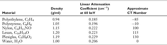
Modified from Bushong S: Radiologic science for technologists, ed 9, St Louis, 2009, Mosby.
Uniformity
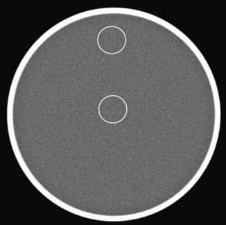
CT number uniformity dictates that for a uniform phantom, the CT number measurement should not change with the location of the selected regions of interest (ROI) or with the phantom position relative to the isocenter of the scanner. For illustration, Figure 9-25 shows a reconstructed 20-cm water phantom. Theoretically, the average CT numbers in two ROI locations should be identical. Because of the effect of beam hardening, scatter, stability of the CT system, and many other factors, the CT number uniformity can only be maintained within a reasonable range (typically 2 HU). As long as the operator understands the system limitations and the factors that influence the performance, he or she can avoid potential pitfalls of using absolute CT numbers for diagnosis.
NOISE
On the basis of the discussion on LCD, the importance of image noise is obvious. Image noise is measured typically on uniform phantoms. To perform noise measurement, the standard deviation, σ, within an ROI of the reconstructed image, f (i, j), is calculated as follows:
where i and j are indices of the two-dimensional image, N is the total number of pixels inside the ROI, and f is the average pixel intensity and is calculated by the following equation:
In both equations, the summation is two dimensional over the ROI. For robustness, several ROIs are often used and the average value of the measured standard deviations is reported.
Noise Sources
Three major sources contribute to the noise in the image. The first source is the quantum noise determined by the x-ray flux or the number of detected x-ray photons. It is influenced by the scanning techniques (e.g., x-ray tube voltage, tube current, slice thickness, scan speed, and helical pitch), the scanner efficiency (e.g., detector quantum efficiency, detector geometrical efficiency, amber-penumbra ratio), and patient (e.g., patient size, amount of bones and soft tissues in the scanning plane). The scanning technique dictates the number of x-ray photons that reach the patient, and the scanner efficiency determines the percentage of the x-ray photons exiting the patient converted to useful signals. The LCD section briefly discusses the tradeoffs of different acquisition parameters. As long as the tradeoffs are well understood, these options can be used effectively to combat noise. More advanced scanners offer features that allow the operator to select a noise level, and the CT system will determine the x-ray tube current required to achieve a specified noise level. Because the patient anatomy changes with location, the x-ray tube current typically changes as a function of tube angle as well as the location along the patient long axis.
The second source that influences the noise performance is the inherent physical limitations of the system. These include the electronic noise in the detector photodiode, the electronic noise in the data acquisition system (DAS), scattered radiation, and many other factors. Figure 9-26 shows an oval phantom scanned with two different DAS’s while all other acquisition parameters were kept constant. Significant reduction in image noise can be observed with the lower-noise DAS.
The third noise-influencing factor is the reconstruction parameters. In general, a high-resolution reconstruction kernel produces an increased noise level. This is mainly because these kernels preserve or enhance high-frequency contents in the projection. Unfortunately, most noise presents itself as high-frequency signals. An example of the impact of filter kernel selection on noise is shown in Figure 9-8. Note that the noise level of Figure 9-8, B, is significantly higher than in Figure 9-8, A.
Noise Power Spectrum
It should be pointed out that standard deviation alone is insufficient to fully characterize the noise in the image. This is because noise in the reconstructed images is no longer white. This characteristic can be described by the noise power spectrum, or Wiener spectrum (Riederer et al, 1978). Figure 9-27 shows that the noise power spectrum is obtained with the Fourier transform to break down the image noise into its frequency components. To illustrate the impact of noise spectrum on the image, Figure 9-28 shows a low-contrast phantom scanned with different tube currents and reconstructed with different kernels, one with the standard kernel and the other with the bone kernel. The tube currents were selected such that both images have the same standard deviation. However, the visibility of the low-contrast objects is clearly different. This demonstrates the importance of the fact that, to fully characterize the noise in the image, standard deviation alone is insufficient.
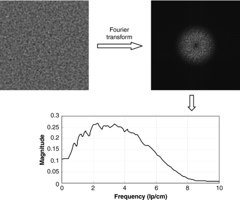
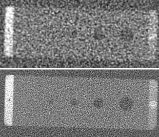
IMAGE ARTIFACT
Definition and General Discussion
Artifacts can degrade image quality, affect the perceptibility of detail, or even lead to misdiagnosis. This can cause serious problems for the radiologist who has to provide a diagnosis from images obtained by the technologist. Therefore it is mandatory that the technologist understand the nature of artifacts in CT.
In general, an artifact is “a distortion or error in an image that is unrelated to the subject being studied” (Morgan, 1983). Specifically, a CT image artifact is defined as “any discrepancy between the reconstructed CT numbers in the image and the true attenuation coefficients of the object” (Hsieh, 1995). This definition is comprehensive and implies that anything that causes an incorrect measurement of transmission readings by the detectors will result in an image artifact. Because CT numbers represent gray shades in the image, incorrect measurements will produce incorrect CT numbers that do not represent the attenuation coefficients of the object. These errors result in various artifacts that affect the appearance of the CT image.
In CT, artifacts arise from a number of sources, including the patient, inappropriate selection of protocols, reconstruction process, problems relating to the equipment such as malfunctions or imperfections, and fundamental limitation of physics. In a typical commercial CT system, an image is reconstructed from 106 independent projection samples. The contribution of each projection reading, on the other hand, is not limited to an isolated point in the reconstructed image as a result of the convolution and back-projection process discussed in Chapter 6. This is a radical departure from conventional radiographic imaging, in which each measured sample affects only the value of a single pixel in the resulting image. As a result, the probability of an artifact for CT is significantly higher compared with the conventional radiograph. Given the numerous sources of artifacts and the complexity of the artifact manifestation, it is impossible to cover this topic in a short section. This chapter focuses, instead, on the most important artifacts in routine clinical applications. Interested readers can refer to Hsieh (2003) for more comprehensive coverage on this topic.
Types and Causes
Artifacts in CT can be classified according to cause and appearance. In the classification of artifacts on the basis of their appearance in the image, four major categories can be identified, including streaks, shadings, rings and bands, and “miscellaneous” factors such as the basket weave and moiré patterns (Fig. 9-29) (Table 9-2). Streak artifacts may appear as intense straight lines across an image, which may be caused by improper sampling of the data (aliasing), partial volume averaging, motion, metal, beam hardening, noise, spiral/helical scanning, and mechanical failure or imperfections. Streak artifacts are often caused by errors of isolated projection readings (isolated channels and views). These discrepancies are enhanced by the convolution process and manifested into lines during the back-projection, as shown in Figure 9-29, A.
TABLE 9-2
Classification of Artifacts on the Basis of Appearance
| Appearance | Cause |
| Streaks | Improper sampling of data; partial volume averaging; patient motion; metal; beam hardening; noise; spiral/helical scanning; mechanical failure |
| Shading | Partial volume averaging; beam hardening; spiral/helical scanning; scatter radiation; off-focal radiation; incomplete projections |
| Rings and bands | Bad detector channels in third-generation CT scanners |
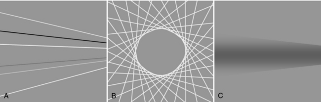
Ring or band artifacts are produced when the projection readings of a single channel or a group of channels consistently deviate from the truth. The can be the result of defective detector cells or DAS channels, deficiencies in system calibration, or a suboptimal image-generation process. This is predominately a third-generation CT scanner phenomenon. Because a detector channel reading is always mapped to a straight line that is at a fixed distance to the isocenter of the system, a defective reading forms a ring pattern during the back-projection process, as illustrated in Figure 9-29, B.
Shading artifacts often appear near objects of high densities and can be caused by beam hardening, partial volume averaging, spiral/helical scanning, scatter radiation, off-focal radiation, and incomplete projections. They are formed by the gradual deviation of a group of projection readings over a limited range of views, as shown in Figure 9-29, C.
Common Artifacts and Correction Techniques
Patient Motion Artifacts: Patient motion can be voluntary or involuntary. Voluntary motion is directly controlled by the patient, such as swallowing or respiratory motion. Involuntary motion is not under the direct control of the patient, such as head motion with injury, peristalsis, and cardiac motion, as shown in Figures 9-30, A, and 9-31, A. Both voluntary and involuntary motions appear as streaks that are usually tangential to high-contrast edges of the moving part. Additionally, motion artifacts can arise from movement of oral contrast in the gastrointestinal tract.
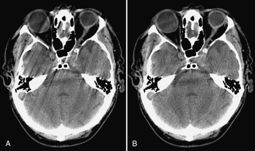
FIGURE 9-30 Illustration of patient involuntary head motion. A, Without compensation. B, With correction.
The appearance of streaks results from the inability of the reconstruction algorithm to deal with data inconsistencies in voxel attenuation arising from the edge of the moving part. There are several methods to reduce CT artifacts from motion. For patient movements such as breathing and swallowing, it is important to immobilize patients and use positioning aids to make them comfortable and to ensure that patients understand the importance of remaining still and following instructions during scanning. Another useful motion artifact reduction technique is to shorten the scan time, as discussed in the temporal resolution section of this chapter. Correction of motion artifacts can also be accomplished with software such as underscan weighting, as shown in Figures 9-30, B, and 9-31, B (Hsieh, 2003), and physiological gating such as ECG-gated cardiac, as demonstrated in Figure 9-21.
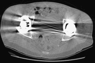
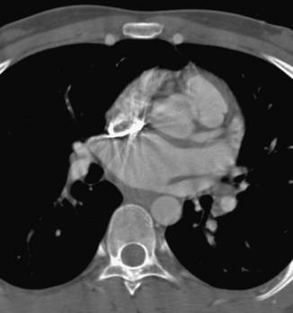
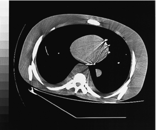
Metal Artifacts: The presence of metal objects in the patient also causes artifacts. Metallic materials such as prosthetic devices, dental fillings, surgical clips, and electrodes give rise to streak artifacts on the image (Fig. 9-32). The creation of these artifacts and a method of correction are illustrated in Figure 9-33. As shown in Figure 9-33, A, the metal object is highly attenuating to the radiation, which results in significant error in projection profiles. The error is the combined effects of signal underrange, beam hardening, partial volume, and limited dynamic range of the acquisition and reconstruction systems. The loss of information leads to the appearance of typical star-shaped streaks. It should be pointed out that patient motion is often a major culprit in exacerbating the appearance of artifacts, as illustrated in Figure 9-34 with a pacemaker lead in a patient’s heart.
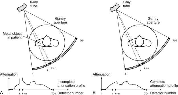
Metal artifacts can be reduced by the removal of all external metal objects from the patient. Software such as the metal artifact reduction (MAR) program can be used to complete the incomplete profile through interpolation (Fig. 9-33, B). The procedure is described as follows (Felsenberg et al, 1988):
1. Acquisition and storage of the raw data
2. Reconstruction of a CT image
3. Identification of the implant
4. Automatic definition of the boundaries of the implant within the projection data. For each projection, the implant boundaries are automatically defined within the given ROI by the use of given threshold values.
5. Linear interpolation of the missing projection data
6. Reconstruction of the artifact-reduced image from the newly computed projection data
It should be pointed out that, although metal artifact correction has been the focus of many studies over decades, an effective and robust method is yet to be found. This is due not only to the complexity of the problem (e.g., different type and shape of metals, patient motion, and partial volume), but also to the challenging clinical needs. Radiologists are often interested in the region immediately adjacent to the metal implant to assess the patient condition. Many correction methods, such as the one outlined previously, do not preserve the integrity of such regions.
Beam-Hardening Artifacts: Beam hardening refers to an increase in the mean energy of the x-ray beam as it passes through the patient. As the object size increases, the mean energy shifts to the right because lower energy photons are absorbed preferentially as the beam passes through the object. For illustration, we depict the original x-ray tube spectrum, the spectrum after traversing 15 cm water, and the spectrum after traversing 30 cm water (Figure 9-35). For each graph, the number of detected x-ray photons is kept to one million. Note that as the x-ray spectrum is modified, the CT numbers of certain structures change. Additionally, because radiation beams have different path lengths through the object (Fig. 9-36), the x-ray beam spectrum becomes channel dependent. The top portion of Figure 9-36 shows a short and a long path length, which results in different degrees of beam hardening. There is less beam hardening at the periphery of the object, where the radiation path is short, compared with the center of the object, where the radiation path is longer. The bottom portion of Figure 9-36 depicts the intensity profiles of the reconstructed images. Ideally, the intensity should be constant for a uniform object, as shown by the thick solid line. Because of the beam-hardening effect, errors in CT numbers increase gradually from the periphery to the center of the object, as depicted by the dotted line. This artifact can be corrected by performance of a polynomial mapping of the measured projections before the reconstruction (Hsieh, 2003). Figure 9-37 shows two reconstructed images of a 35-cm water phantom with (B) and without (A) beam-hardening correction.
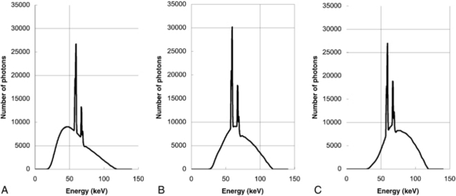
FIGURE 9-35 Effect of beam hardening as the x-ray beam traverses different object sizes. A, Original spectrum. B, After traversing 15 cm water. C, After traversing 30 cm water.
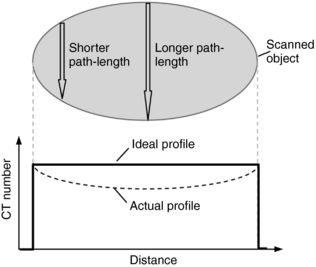
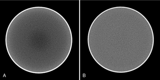
FIGURE 9-37 Reconstructed images of a 35-cm water phantom. A, Without beam-hardening correction. B, With beam-hardening correction.
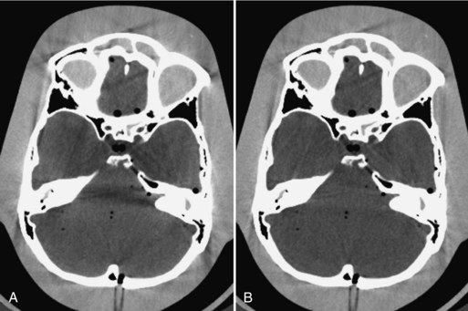
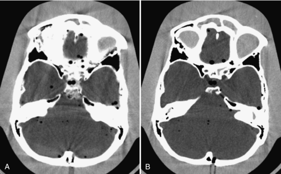
The beam-hardening effect is material dependent. When dense bones or contrast agents are present in the beam path, dark shading artifacts can result because the beam-hardening correction applied to soft tissue does not work well for bones. This effect is demonstrated in Figure 9-38, A. Note the dark banding connecting the temporal bones. It has been shown that iterative correction is effective in combating such artifacts, as shown by Figure 9-38, B (Joseph and Ruth, 1997).
Partial Volume Artifacts: CT numbers are based on the linear attenuation coefficients for a voxel of tissue. If the voxel contains only one tissue type, the calculation will not be problematic. For example, if the tissue in the voxel is gray matter, the CT number is computed at around 43. If the voxel contains three similar tissue types in which the CT numbers are close together—for example, blood (CT number 40), gray matter (43), and white matter (46)—then the CT number for that voxel is based on an average of the three tissues. This is known as partial volume averaging.
When the voxel contains multiple materials that are significantly different (e.g., soft tissue and bone), partial volume averaging can lead to partial volume artifacts (Heuscher and Vembar, 1999). In Figure 9-39, A, the detector measures x-ray intensity transmitted from the bone, I1, and soft tissue, I2, at the same time. Mathematically, the total intensity is measured as I1 + I2. To convert from intensities to line integrals for reconstruction, it is necessary to perform the logarithmic operation. Because of the nonlinear nature of the operator, it is clear that:
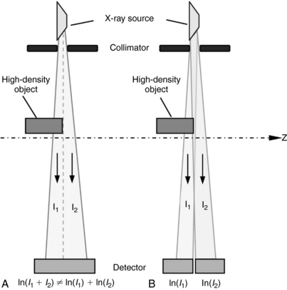
FIGURE 9-39 Cause and correction for partial volume effect. A, Nonlinear operation of logarithm. B, Thin slice scanning.
These inaccuracies result in partial volume artifacts in the image, which appear as bands and streaks (Fig. 9-40, A).
Partial volume artifacts can be reduced with thinner slice acquisitions and computer algorithms (Hsieh, 1995). It is interesting to note that the thin-slice data acquisition comes naturally with the multislice CT. When the two intensities, I1 and I2, are measured with two separate detector cells, as shown in Figure 9-39, B, the object within each slice width is uniform and logarithm operation is performed on the two intensities individually. Figure 9-40, B, shows the same phantom scanned with a thinner slice; the partial volume artifacts are nearly eliminated.
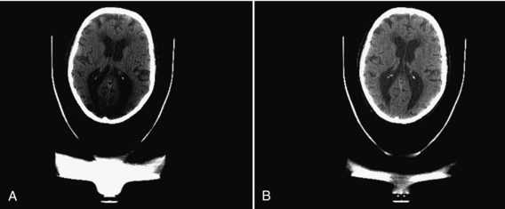
It is worth pointing out that partial volume artifacts can occur even with thin-slice acquisition if special attention is not paid to other accessories near the patient. As an example, Figure 9-41, A, shows a patient head supported by a high-density extension that ends abruptly at the mid brain location. Because of the sharp structure of this particular device, even a 1-mm slice thickness is insufficient to avoid partial volume artifacts, as demonstrated by the severe shading at the lower portion of the brain. Note that an adjacent slice (B), which is located 1 mm apart, is free from such artifacts because the supporting structure becomes homogeneous within this slice.
Aliasing Artifacts: The sampling theorem states that to faithfully represent a continuous signal (e.g., intensity profile of a patient), the sampling frequency fN (the number of rays/cm in the fan beam) must be at least twice the highest frequency content in the signal, fH. Mathematically, this can be expressed as follows:

If this criterion, the Nyquist criterion, is not met, aliasing artifacts (streaks) can result after the reconstruction process. During CT data acquisition, the original continuous signal is sampled to a discrete form both spatially (each projection is sampled by multiple detector channels) and temporally (each data acquisition is divided into multiple views). Consequently, aliasing artifacts can arise from insufficient projection sampling or from insufficient view sampling. For illustration, Figure 9-42 shows a torso phantom that was scanned with half the normal number of views.

FIGURE 9-42 View aliasing artifacts resulting from 50% of the normal number of views used to scan this torso phantom. The artifacts are apparent at the periphery of the phantom.
Various methods are available to minimize aliasing artifacts. In some cases the number of views or number of ray samples per view can be increased (Fig. 9-43) to meet the Nyquist requirements. The convolution kernel used in the reconstruction can also be modified so that only frequencies below the Nyquist frequency are allowed into the filtered projection. In this case, a tradeoff is made between the aliasing artifact reduction and spatial resolution of the reconstructed image.
Noise-Induced Artifacts: Noise is influenced partially by the number of photons that strike the detector. Photon starvation can occur as a result of poor patient positioning in the scan SFOV and poor selection of exposure techniques (peak kV, mA), scan speed, and limitations of the CT scanner such as maximum tube power. More photons mean less noise and a stronger detector signal, whereas fewer photons result in more noise and a weaker detector signal. When it is combined with the electronic noise and the logarithmic operation, photon starvation often leads to severe streak artifacts, as shown in Figure 9-44, A.
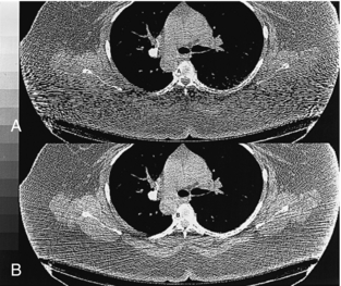
FIGURE 9-44 A, Streak artifacts can arise from an increase in noise resulting from reduced photons at the detector. B, Correction of the streaks by adaptive filtering.
The technologist should optimize patient positioning, scan speed, and exposure technique factors to correct streak artifacts. These artifacts can also be reduced with adaptive filtering algorithms (Fig. 9-44, B). These algorithms dynamically adjust the amount of smoothing operation on the basis of the x-ray flux level at each projection channel. By selectively smoothing only the channels that contribute to the streaking artifacts and by varying the degree of smoothing on the basis of the noise level of the signal, the technologist can achieve the objectives of simultaneously reducing the streak artifacts in the images and preserving the spatial resolution of the system (Hsieh, 1998).
Another type of the noise-induced artifact is related to the noise nonuniformity. When the noise within the reconstruction FOV is highly heterogeneous, it can produce bright and dark horizontal strips in the MIP or VR images, as shown in Figure 9-45, A. This type of artifact can be reduced with either an improved reconstruction algorithm or advanced image processing. Both approaches produce a more uniform noise pattern in the final image (Fig. 9-45, B).
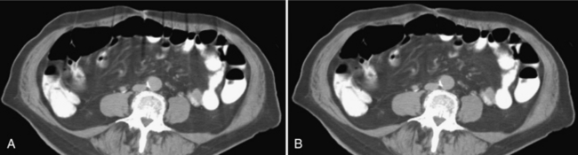
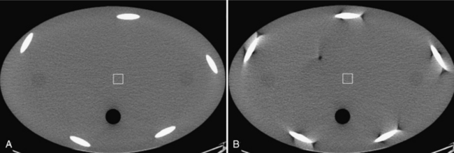
Scatter: Scattered radiation is a fundamental phenomenon associated with the interaction between x-ray photons and matter. It reduces the object contrast in conventional radiography and produces artifacts in CT. Scattered radiation has been controlled effectively in the past by placing a postpatient collimator in front of the detector to reject any photons that do not follow the straight-line path between the x-ray source and the detector cell. With the introduction of multislice and volumetric CT, the volume that is exposed to the x-ray radiation increases significantly while the detector aperture reduces. As a result, the scatter-to-primary ratio (ratio of the scattered signal versus true signal) increases. The one-dimensional collimator plates are no longer sufficient, as demonstrated by Figure 9-46, A. Note the dark shading artifacts connecting the dense rods.
Scatter-induced artifacts can be corrected with algorithms by carefully measuring or estimating the scatter distribution in the projection. The estimated scatter can then be removed from the measured intensities to arrive at the true signals that represent the line integrals of the scanned object. Figure 9-46, B, depicts the same scan reconstructed with a software scatter correction. A uniform background is restored.
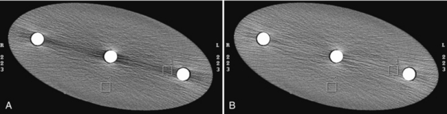
Cone-Beam Artifacts: The cone-beam artifact is a complicated subject. It is impossible to cover this topic in a subsection. At a very high level, cone-beam artifacts are caused by incomplete or insufficient projection samples as a result of the cone-beam geometry of multislice CT. Understanding the subject involves discussions of the cone-beam reconstruction theory. Given the limited scope of this section, this chapter only provides a specific example of the cone-beam artifact produced with one of the popular reconstruction algorithms: FDK algorithm (Feldkamp et al, 1984). For illustration, a simulation of a helical body phantom is scanned in a step-and-shoot mode with a 64 × 0.625 mm detector configuration (Tang et al, 2005). The comparison of a relatively centered slice (Fig. 9-47, A) and an edge slice (Fig. 9-47, B) shows both distortions of the dense oval objects as well as shading artifacts nearby. The dense oval objects are ellipsoids positioned at a steep angle with respect to the patient’s long axis to accentuate the artifacts. Reduction and elimination of cone-beam artifacts have been the focus of intense investigations in recent years, and this research will likely continue for years to come.
QUALITY CONTROL
Quality control is an integral part of equipment testing and maintenance programs in hospitals. Quality control ensures the optimal performance of the CT scanner through a series of daily, monthly, and annual tests for spatial resolution, contrast resolution, noise, slice width, peak kV waveform, average CT number of water, standard deviation of CT numbers in water, and radiation scatter and leakage. These tests constitute a general quality control program for CT scanners and need to be documented.
REFERENCES
Barnes, GT, Lakshminarayanan, AV. Computed tomography: physical principles and image quality considerations. In Lee JK, et al, eds.: Computed tomography with MRI correction, 2, New York: Raven Press, 1981.
Blumenfeld, SM, Glover, G. Spatial resolution in computed tomography. In: Newton, TH, Potts, DG, eds. Radiology of the skull and brain: technical aspects of computed tomography, 5. St Louis: Mosby; 1981.
Bushong, S. Radiologic science for technologists, 9. St Louis: Mosby, 2009.
Curry, TS, et al. Christensen’s physics of diagnostic radiology, 4. Philadelphia: Lea & Febiger, 1990.
Feldkamp, LA, et al. Practical cone-beam algorithm. J Opt Soc Am. 1984;1:612–619.
Felsenberg, D, et al. Reduction of metal artifacts in computed tomography-clinical experience and results. Electromedica. 1988;56:97–104.
Goodenough, DJ, et al. Development of a phantom for evaluation and assurance of image quality in CT scanning. Opt Eng. 1977;16:52–65.
Hanson, KM. Noise and contrast and discrimination in computed tomography. In: Newton, TH, Potts, DG, eds. Radiology of the skull and brain: technical aspects of computed tomography, 5. St Louis: Mosby; 1981.
Heuscher, DJ, Vembar, M. Reduced partial volume artifacts using spiral computed tomography and integrating spiral interpolator. Med Phys. 1999;26:276–287.
Hounsfield, GN. Potential uses of more accurate CT absorption values by filtering. AJR Am J Roentgenol. 1978;131:103–106.
Hsieh, J. Image artifacts, causes and correction. In: Goldman LW, Fowlkes JB, eds. Medical CT and ultrasound: current technology and applications. College Park, Md: American Association of Physicists in Medicine, 1995.
Hsieh, J. Adaptive artifact reduction in computed tomography resulting from x-ray photon noise. Med Phys. 1998;25:2139–2147.
Hsieh, J. Investigation of the slice sensitivity profile for step-and-shoot mode multi-slice CT. Med Phys. 2001;28:491–500.
Hsieh, J. Computed tomography: principles, design, artifacts, and recent advances. Seattle: SPIE Press, 2003.
Hsieh, J, et al. Non-uniform phase coded image reconstruction for cardiac CT. Radiology. 1999;213:401–406.
Joseph, PM, Ruth, C. Method for simultaneous correction of spectrum hardening artifacts in CT images containing both bone and iodine. Med Phys. 1997;24:1629–1643.
Kachelriess, M, et al. ECG-correlated imaging of the heart with subsecond multislice spiral CT. IEEE Trans Med Imag. 2000;19:888–901.
Kalender, WA, Polacin, A. Physical performance characteristics of spiral CT scanning. Med Phys. 1991;18:910–915.
Mayo, JR. High-resolution computed tomography: technical aspects. Radiol Clin North Am. 1991;29:1043–1048.
McCollough, CH, Zink, FE. Performance evaluation of CT systems. In: Goldman LW, Fowlkes JB, eds. Categorical courses in diagnostic radiology physics: CT and US cross-sectional imaging. Oak Brook, Ill: Radiological Society of North America; 2000:189–207.
Morgan, CL. Basic principles of computed tomography. Baltimore: University Park Press, 1983.
Parker, DL. Optimal short scan convolution reconstruction for fan-beam CT. Med Phys. 1982;9:254–257.
Pfeiler, M, et al. Some guiding ideas on image recording in computerized axial tomography. Electromedica. 1976;1:19–25.
Riederer, SJ, et al. The noise power spectrum in computer x-ray tomography. Phys Med Biol. 1978;23:446–454.
Robb, RA, Mortin, RL. Principle and instrumentation for dynamic x-ray computed tomography. In: Marcus ML, et al, eds. Cardiac imaging: a comparison to Braunwald’s heart disease. Philadelphia: WB Saunders, 1991.
Tang, XY, et al. A three-dimensional weighted cone beam filtered backprojection (CB-FBP) algorithm for image reconstruction in volumetric CT under a circular source trajectory. Phys Med Biol. 2005;50:3889–3905.