Image Reconstruction
BASIC PRINCIPLES
For the computer to reconstruct an image of the patient by computed tomography (CT), the x-ray tube and detectors must rotate around the patient for at least 180 degrees. In this way, sufficient x-ray transmission values or attenuation data are collected to satisfy the image reconstruction process that builds up an image of acceptable quality. The reconstruction process is based on the use of an algorithm that uses the attenuation data measured by the detectors to systematically build up the image for viewing and interpretation. The sequence of events after the data are collected from the detectors is shown in Figure 6-1. Although the older CT scanners collected data over 180 degrees, present-day CT scanners collect more attenuation data over 360 degrees to generate better-quality images. The image reconstruction algorithms, as they are referred to, are numerous and have been developed and subsequently modified to meet the requirements of the new generation of CT scanners. Understanding these algorithms requires a basic introduction to several concepts, including the Fourier transform, convolution, and interpolation.
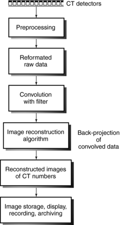
FIGURE 6-1 Sequence of events after signals leave the detectors. The image reconstruction algorithms deal with the mathematics of the CT process.
The purpose of this chapter is to present a brief nonmathematical description of several image reconstruction algorithms with the goal of impressing on the technologist that the problem in CT is a mathematical one and therefore mathematical solutions are needed to solve the problem. The description will begin with the algorithms used in the earlier conventional CT scanners, followed by a brief introduction to the algorithms used in single-slice spiral/helical CT (SSCT) and multislice spiral/helical CT (MSCT) scanners. The latter is described in more detail in later chapters dealing with SSCT and MSCT scanning principles.
Algorithms
The algorithm is now common in radiology because computers are used in many imaging and nonimaging applications. The word algorithm is derived from the name of the Persian scholar, Abu Ja’Far Mohammed ibn Mûsâ Alkowârîzmî, whose textbook on arithmetic (c. 825 CE) significantly influenced mathematics for many years (Knuth, 1977). According to Knuth, an algorithm is “a set of rules or directions for getting a specific output from a specific input. The distinguishing feature of an algorithm is that all vagueness must be eliminated; the rules must describe operations that are so simple and well defined, they can be executed by a machine. Furthermore, an algorithm must always terminate after a finite number of steps.”
The solutions to mathematical problems in CT require image reconstruction algorithms, available as computer software to reconstruct the image.
Fourier Transform
The Fourier transform, which was developed by the mathematician Baron Jean-Baptiste-Joseph Fourier in 1807, is widely used in science and engineering. The Fourier transform is a useful analytical tool in mathematics, astronomy, chemistry, physics, medicine, and radiology. In radiology, the Fourier transform is used to reconstruct images of a patient’s anatomy in CT and also in magnetic resonance imaging (MRI).
To understand the Fourier transform, Bracewell (1989) presented an analogy with the act of hearing. Incoming sound waves that enter the ear are separated into different signals and intensities. These signals arrive at the brain and are rearranged to produce a perception of the original sound. Bracewell defined the Fourier transform as “a function that describes the amplitude and phases of each sinusoid, which corresponds to a specific frequency. (Amplitude describes the height of the sinusoid; phase specifies the starting point in the sinusoid’s cycle.)” In other words, the Fourier transform is a mathematical function that converts a signal in the spatial domain to a signal in the frequency domain.
The Fourier transform divides a waveform (sinusoid) into a series of sine and cosine functions of different frequencies and amplitudes. These components can then be separated. In imaging, when a beam of x rays passes through the patient, an image profile denoted by f(x) is obtained. This can be expressed mathematically in the form of the Fourier series as follows:
The constants—a0, a1, b1, and so on—are called Fourier coefficients (Gibson, 1981) and can easily be calculated. Use of these Fourier coefficients makes it possible to reconstruct an image in CT.
Convolution
Convolution is a digital image processing technique to modify images through a filter function (see Chapter 3). “The process involves multiplication of overlapping portions of the filter function and the detector response curve selectively to produce a third function which is used for image reconstruction” (Berland, 1987). (This will become clear in the discussion of the filtered back-projection algorithm.)
Interpolation
Interpolation is used in CT in the image reconstruction process and the determination of slices in spiral/helical CT imaging. Interpolation is a mathematical technique to estimate the value of a function from known values on either side of the function.
For example, if the speed of an engine controlled by a lever increases from 40 to 50 revolutions per second when the lever is pulled down by 4 cm, one can interpolate from this information and assume that moving it 2 cm gives 45 revolutions per second. This is the simplest method of interpolation, called linear interpolation. If known values of one variable, Y, are plotted against the other variable, X, an estimate of an unknown value of Y can be made by drawing a straight line between the two nearest known values. The mathematical formula for linear interpolation is

where Y3 is the unknown value of Y (at X3) and Y2 and Y1 (at X2 and X1) are the nearest known values between which the interpolation is made (Gibson, 1981).
IMAGE RECONSTRUCTION FROM PROJECTIONS
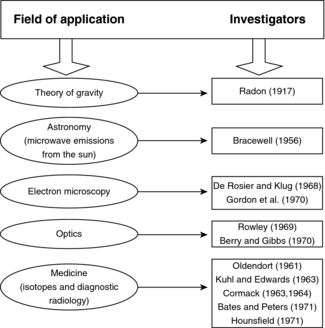
The history of reconstruction techniques dates to 1917 when Radon developed mathematical solutions to the problem of image reconstruction from a set of its projections. He applied these techniques to gravitational problems. These techniques were later used to solve problems in astronomy and optics, but they were not applied to medicine until 1961 (Fig. 6-2).
In his initial work, Hounsfield’s images were noisy as a result of his chosen reconstruction technique. Special algorithms (convolution back-projection algorithms) were soon introduced. These algorithms were developed by Ramachandran and Lakshminarayanan (1971) and later used by Shepp and Logan (1974) to improve image quality and processing time.
Problem in CT
Consider an object, O, represented by an x-y coordinate system (Fig. 6-3). The spatial distribution of all attenuation coefficients, μ, is given by μ(x,y), which varies between points in the object. Suppose a pencil beam of x rays passes through the object along a straight path (arrow), and the intensity of the transmitted beam that falls on the CT detector is I. Then a projection is given by the line integral* of μ(x,y):
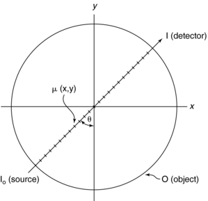
FIGURE 6-3 The total distribution of attenuation coefficients in the object O is μ(x,y). The problem in CT is to calculate μ(x,y) from a set of projections specified by the angle θ. I0 and I represent beam intensities from the source and at the detector, respectively. From Seeram E: Computed tomography technology, Philadelphia, 2001, WB Saunders.
By taking the negative logarithm, Equation 6-1 can be linearized to generate integral equations of the form
where Tθ(x) is the x-ray transmission at angle θ, which is a measure of the total absorption along the straight line in Figure 6-3. Tθ(x) is referred to as the ray sum, which is the integral of μ(x,y) along the ray.
The computational problem in CT is to find μ(x,y) from the ray sums for a sufficiently large number of beams of known locations that pass through the object, O. The beam geometries discussed in Chapter 5 ensure that every point in the object is scanned successively by a large set of ray sums Tθ(x).
A set of ray sums is referred to as a projection (Fig. 6-4), which can be generated as shown in Figure 6-4, as the x-ray tube and detector scan the object simultaneously. The ray AA′ is equal to x cos θ + y sin θ = d. The projection is given by P(θ,d):
where ds is the differential along the path length s.
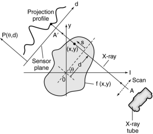
FIGURE 6-4 Projection profile obtained when a parallel beam of x rays scans the object represented by f(x,y). (d is the distance of the ray AA′ from the origin 0).
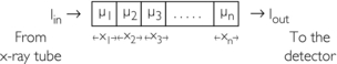
To understand the meaning of a projection, consider the following case in which a beam of intensity Iin enters an object of thickness x:
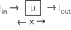
The beam is attenuated according to Lambert-Beer’s law, as follows:
Because x, Iin, Iout, and e are known, μ can be calculated:
The following case represents the situation in the patient:

The problem in CT is to calculate all values for the μ terms for a large set of projections. Projections can be obtained through both parallel and fan beam geometries (Fig. 6-5). Hounsfield’s original CT scanner used parallel beam projections acquired through a 180-degree rotation.
RECONSTRUCTION ALGORITHMS
Image reconstruction from projections involves several algorithms to calculate all the μ terms in Equation 6-7 from a set of projection data. The algorithms applicable to CT include back-projection, iterative methods, and analytic methods.
Back-Projection
Back-projection is a simple procedure that does not require much understanding of mathematics. Back-projection, also called the “summation method” or “linear superposition method,” was first used by Oldendorf (1961) and Kuhl and Edwards (1963). Back-projection can be best explained with a graphical or numerical approach.
Consider four beams of x rays that pass through an unknown object to produce four projection profiles P1, P2, P3, P4 (Fig. 6-6). The problem involves the use of these profiles to reconstruct an image of the unknown object (black dot) in the box. The projected data sets are back-projected (i.e., linearly smeared) to form the corresponding images BP1, BP2, BP3, and BP4. The reconstruction involves summing these back-projected images to form an image of the object.
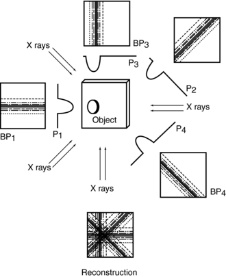
The problem with the back-projection technique is that it does not produce a sharp image of the object and therefore is not used in clinical CT. The most striking artifact of back-projection is the typical star pattern that occurs because points outside a high-density object receive some of the back-projected intensity of that object (Curry et al, 1990).
Back-projection can also be explained with the following 2 × 2 matrix:
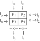
Four separate equations can be generated for the four unknowns, μ1, μ2, μ3, and μ4:
A computer can solve these equations very quickly.
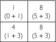
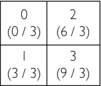
A numerical example might help to give some insight into the calculations involved. Consider an object divided into four squares (2 × 2 matrix with four pixels), as shown on the follwing page.
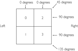
Four projections are collected at four different known locations: 0, 45, 90, and 135 degrees.
To start, data are collected for four projections: 0, 45, 90, and 135 degrees.
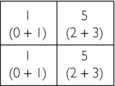
1. The ray sum for the 0-degree projection on the left side is 1 (0 + 1).
2. The ray sum for the 0-degree projection on the right side is 5 (2 + 3).
3. The ray sums for the 45-degree projection are 0, 3 (2 + 1), and 3.
4. The ray sum for the 90-degree projection on the upper row is 2 (2 + 0).
5. The ray sum for the 90-degree projection on the lower row is 4 (3 + 1).
6. The ray sums for the 135-degree projection are 2, 3 (3 + 0), and 1.
These projection data—1, 5, 0, 3, 3, 2, 4, 2, 3, and 1—are then used systematically as defined by the algorithm to reconstruct the original image.
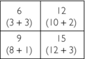
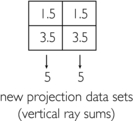
1. First guess: Place the data from the 0-degree projections into the matrix to obtain the first guess:
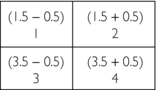
2. Second guess: Add the data from the 45-degree projections to the value of each square in the first guess:
3. Third guess: Add the data from the 90-degree projections to the value of each square in the second guess:
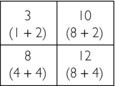
4. Fourth guess: Add the data from the 135-degree projections to the value of each square in the third guess:
Iterative Algorithms
Another approach to image reconstruction is based on iterative techniques. “An iterative reconstruction starts with an assumption (for example, that all points in the matrix have the same value) and compares this assumption with measured values, makes corrections to bring the two into agreement, and then repeats this process over and over until the assumed and measured values are the same or within acceptable limits” (Curry et al, 1990).
Techniques include the simultaneous iterative reconstruction technique, the iterative least-squares technique, and the algebraic reconstruction technique (Brooks and Di Chiro, 1976; Gordon and Herman, 1974). These techniques differ in the application of corrections to subsequent iterations. The algebraic reconstruction technique was used by Hounsfield in the first EMI brain scanner (Hounsfield, 1972) and is detailed here.
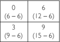
Consider the following numeric illustration:
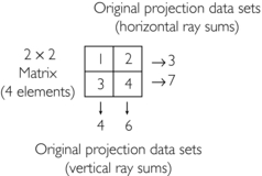
1. Initial estimate: Compute the average of four elements and assign it to each pixel, that is, 1 + 2 + 3 + 4 = 10; 10/4 = 2.5
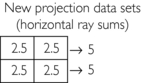
2. First correction for error (original horizontal ray sums minus the new horizontal ray sums divided by 2) = (3−5) / 2 and (7−5) / 2 = −2 / 2 and 2/2 = −1.0 and 1.0:
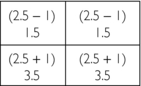
4. Second correction for error (original vertical ray sums minus new vertical ray sums divided by 2) = (4−5) / 2 and (6−5) / 2 = −1.0/2 and +1.0/2 = −0.5 and +0.5:
The final matrix solution is thus

Today these techniques are not used in commercial scanners because of the following limitations:
1. It is difficult to obtain accurate ray sums because of quantum noise and patient motion.
2. The procedure takes too long to generate the reconstructed image because the iteration can be done only after all projection data sets have been obtained.
3. To produce a “true” image, there should be more projection data sets than pixels. Therefore diagonal projection data sets are taken to eliminate ambiguity.
Analytic Reconstruction Algorithms
Analytic reconstruction algorithms were developed to overcome the limitations of back-projection and iterative algorithms and are used in modern CT scanners. Two analytic reconstruction algorithms are the Fourier reconstruction algorithm and filtered back-projection.
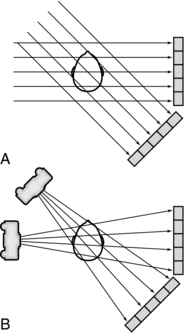
Filtered Back-Projection: Filtered back-projection is also referred to as the convolution method (Fig. 6-7). The projection profile is filtered or convolved to remove the typical starlike blurring that is characteristic of the simple back-projection technique.
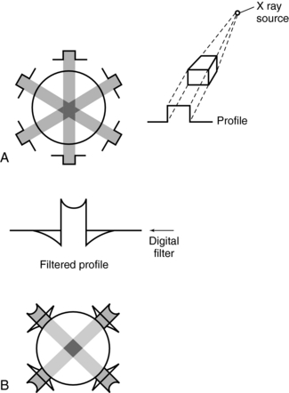
FIGURE 6-7 Back-projection and filtered back-projection techniques used in CT. A, Back-projection results in an unsharp image. B, Filtered back-projection uses a digital filter (a convolution filter) to remove this blurring, which produces a sharp image.
The steps in the filtered back-projection method (Fig. 6-7, B) are as follows:
1. All projection profiles are obtained.
2. The logarithm of the data is obtained.
3. The logarithmic values are multiplied by a digital filter, or convolution filter, to generate a set of filtered profiles.
4. The filtered profiles are then back-projected.
5. The filtered projections are summed and the negative and positive components are therefore canceled, which produces an image free of blurring.
Fourier Reconstruction: The Fourier reconstruction process is used in MRI but not in modern CT scanners because it requires more complicated mathematics than does the filtered back-projection algorithm.
A radiograph can be considered an image in the spatial domain; that is, shades of gray represent various parts of the anatomy (e.g., bone is white and air is black) in space. With the Fourier transform, this spatial domain image—the radiograph represented by the function f(x,y)—can be transformed into a frequency domain image represented by the function F(u,v). This frequency domain image consists of a range of high to low frequencies. In addition, this image can be retransformed into a spatial domain image with the inverse Fourier transform (Fig. 6-8).
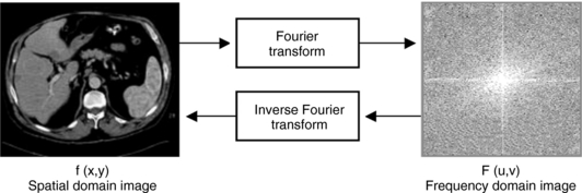
FIGURE 6-8 Radiograph of an image represented in the spatial domain by the function f(x,y). This can be transformed to an image in the frequency domain F(u,v) with use of the Fourier transform. In addition, F(u,v) can be retransformed into f(x,y) with use of the inverse Fourier transform.
There are several advantages to this transformation process. First, the image in the frequency domain can be manipulated (e.g., edge enhancement or smoothing) by changing the amplitudes of the frequency components. Second, a computer can perform those manipulations (digital image processing). Third, frequency information can be used to measure image quality through the point spread function, line spread function, and modulation transfer function (Huang, 1999).
The Fourier slice theorem states that the Fourier transform of the projection of an object at angle θ is equal to a slice of the Fourier transform of the object along angle θ (Fig. 6-9).
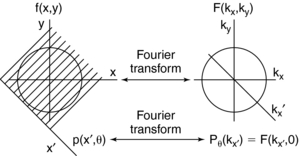
FIGURE 6-9 The projection slice theorem forms the basis of Fourier reconstruction mathematics. The Fourier transform of the projection with respect to x′,Pθ(kx) is equal to a slice of the Fourier transform F(kx,ky) in the θ direction.
The Fourier reconstruction consists of the following steps (Fig. 6-10):
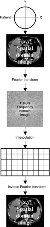
1. The object to be scanned is represented by the function f(x,y).
2. Projection data are obtained from the object. A projection data set for at least a 180-degree rotation is required for adequate reconstruction. These projections represent a spatial domain image.
3. Each projection is transformed into the frequency domain by the Fourier transform. This image must be converted into a clinically useful image.
4. Because CT scanners use a fast Fourier transform developed specifically for digital implementation, the frequency domain image must be placed on a rectangular grid (see Fig. 6-10). This is accomplished by interpolation. The fast Fourier transform requires that the pixels in the grid array be 2, 4, 8, 16, 32, 64, 128, 256, 512, 1024, and so on.
5. Finally, the interpolated image is transformed into a spatial domain image of the object through an inverse Fourier transform operation.
The Fourier reconstruction technique does not use any filtering because interpolation produces a similar result. Also, the two-dimensional (2D) interpolation process may introduce artifacts if it is not conducted accurately; therefore it is not used in CT.
TYPES OF DATA
Figure 6-11 shows the data evolution from acquisition, reconstruction, and image display. Four data types are measurement data, raw data, filtered raw data or convolved data, and image data or reconstructed data.
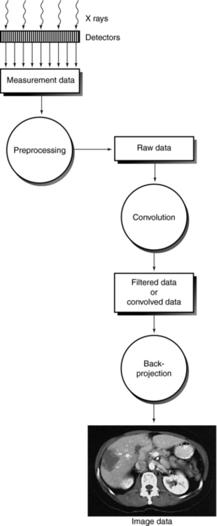
Measurement Data
Measurement data, or scan data, arise from the detectors. This data set is subject to preprocessing to correct the measurement data before the image reconstruction algorithm is applied. Such corrections are necessary because of errors in the measurement data from beam hardening, adjustments for bad detector readings, or scattered radiation. If these errors are not corrected, they will cause poor image quality and generate image artifacts.
Raw Data
Raw data are the result of preprocessed scan data and are subjected to the image reconstruction algorithm used by the scanner. These data can be stored and subsequently retrieved as needed.
Convolved Data
The image reconstruction algorithm used by current CT scanners is the filtered back-projection algorithm, which includes both filtering and back-projection. Raw data must first be filtered with a mathematical filter, or kernel. This process is also referred to as the convolution technique. Convolution improves image quality through the removal of blur (Fig. 6-12). Figure 6-12, A, shows the degree of blurring present in an image before convolution. Figure 6-12, B, demonstrates image sharpening after convolution. Convolution kernels can only be applied to the raw data.

Image Data
Image data, or reconstructed data, are convolved data that have been back-projected into the image matrix to create CT images displayed on a monitor. Various digital filters are available to suppress noise and improve detail (Fig. 6-13). Figure 6-13 shows the relationship between image noise and image detail of a standard algorithm, a smoothing algorithm, and an edge enhancement algorithm.
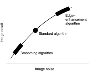
FIGURE 6-13 The relationship between image detail and image noise for three digital filters in CT. Although edge enhancement algorithms provide good detail compared with smoothing algorithms, they also result in more noise. Smoothing algorithms reduce the image noise at the expense of detail but show good soft tissue structures.
The standard algorithm is usually used before the previous algorithms, especially when a balance between image noise and image detail is mandatory. Smoothing algorithms (Fig. 6-14) reduce image noise and show good soft tissue anatomy; they are used in examinations where soft tissue discrimination is important to visualize very low contrast structures. Edge enhancement algorithms emphasize the edges of structures and improve detail but create image noise (see Fig. 6-14). They are used in examinations in which fine detail is important, such as inner ear, bone structures, thin slice, and fine pulmonary structures.
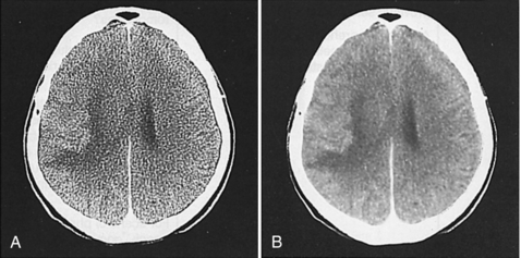
FIGURE 6-14 The effect of two digital filters on the appearance of the CT image. A, An edge enhancement filter is used and more image noise is apparent. B, A smoothing digital filter is used and results in reduced image noise and good soft tissue discrimination. Courtesy Siemens Medical Systems, Iselin, NJ.
IMAGE RECONSTRUCTION IN SINGLE-SLICE SPIRAL/HELICAL CT
The image reconstruction algorithms previously described apply to single-slice conventional CT. In single-slice spiral/helical CT (SSCT), the same filtered back-projection algorithm is used with an additional consideration. Because the patient moves continuously through the gantry for a 360-degree rotation, the reconstructed image will be blurred and therefore interpolation is necessary before the filtered back-projection is used. A planar section must first be computed from the volume data set by using interpolation, after which images are generated with various interpolation algorithms. A more comprehensive description of these algorithms is presented in Chapter 11.
IMAGE RECONSTRUCTION IN MULTISLICE SPIRAL/HELICAL CT
A notable difference between SSCT and multislice spiral/helical CT (MSCT) is that the latter uses multiple detector rows that cover a larger volume at an increased speed and therefore require new algorithms. In general, for CT scanners with four detector rows, MSCT algorithms have been developed to allow for the reconstruction of variable slice thicknesses and address the problems of increased volume coverage and speed of the patient table. This is made possible by spiral/helical scanning with interlaced sampling, longitudinal interpolation, and fan-beam reconstruction with the filtered back-projection algorithm. These three major steps are described further in Chapter 12.
The new generation of MSCT scanners (those with 16 and greater detector rows) require modified image reconstruction algorithms. These algorithms are very complex and beyond the scope of this textbook; however, a few foundational concepts relating to these algorithms are introduced in the next section and further elaborated in Chapter 12, which deals specifically with MSCT principles and concepts.
CONE-BEAM ALGORITHMS FOR THE NEW GENERATION OF MULTISLICE CT SCANNERS
As noted in the chapter so far, a number of image reconstruction algorithms have been developed for conventional “stop-and-go” (or “step-and-shoot”) CT scanners, SSCT scanners, and MSCT scanners with four detector rows.
The types of image reconstruction algorithms and the specific beam geometries characteristic of the new CT scanners are several and are described further in Chapters 11 and 12. Although conventional CT scanners use pencil beam and small fan-beam geometries with the filtered back-projection image reconstruction algorithm, SSCT scanners use wide fan-beam geometries. The image reconstruction algorithm in this case is based on interpolation followed by filtered back-projection. MSCT scanners with four detector rows use a wider fan-beam geometry (compared with SSCT scanners), and therefore use a 2D reconstruction with interpolation and z-filtering, known as z-interpolation algorithms (Chen et al, 2003).
The algorithms for the SSCT and MSCT with four detector rows are referred to as spiral/helical fan-beam approximation algorithms (Hsieh, 2000; Hu, 1999, 2001) simply because they are based on the fan-beam geometry. According to Hein et al (2003), the fan-beam approximation algorithm “assumes that the source, detector, and slice of interest lie in the same plane, and that the projection of the slice of interest falls on a single detector row. This approximation is valid for small cone angles associated with one to four slice systems.” The cone angle is associated with what has been referred to as cone-beam geometry (Flohr et al, 2005).
Cone-Beam Geometry
For a four-detector row MSCT scanner, the beam divergence from the x-ray tube to the outer edges of the detectors increases as shown in Figure 6-15. Such a beam is called a cone beam. Within the cone beam, the rays that will be measured by the detectors are tilted at an angle relative to the central plane (plane perpendicular to the long axis of the patient, the z-axis). This angle is called the cone angle.
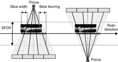
FIGURE 6-15 Diagram shows geometry of four-section CT scanner demonstrating the cone-angle problem: measurement rays are tilted by the so-called cone angle with respect to the center plane. Left and right: Two view angles from sequential scan that are shifted by 180 degrees so that positions of x-ray tube and detector are interchanged. With single-section CT, identical measurement values would be acquired. With multidetector row CT, different measurement values are acquired. SFOV, Scan field of view. From Flohr TG et al: Multi-detector row CT systems and image reconstruction techniques, Radiology 235:756-773, 2005. Reproduced by permission of the Radiological Society of North America and the authors.
As the number of detector rows increases from four to 16 to 64, the cone angle becomes larger. The larger cone angles cause problems where the beam divergence along the z-axis becomes greater. This will result in the plane of interest (planar section of slice of interest) being projected onto several detector rows (Hein et al, 2003). This situation generates inconsistent data that will lead to artifacts called cone-beam artifacts, such as streaking and density changes, both of which will have a negative effect on image quality.
Cone-Beam Algorithms
Fan-beam approximation algorithms require that the data be consistent, that is, the x-ray beam from the tube to the detector, and the section being imaged must be in the same plane. This is no longer the case for large cone angles characteristic of MSCT systems with larger than four detector rows. The fan-beam approximation algorithms are not very accurate for use with the new generation of MSCT scanners, and therefore other image reconstruction algorithms are needed. These algorithms are called cone-beam algorithms, and they have been developed to eliminate the cone-beam artifacts mentioned above. One such popular algorithm is the adaptive multiple plane reconstruction algorithm (Bruening and Flohr, 2003).
Essentially, several cone-beam algorithms have become available for use with the new generation of MSCT scanners, and they basically fall into two classes; exact cone-beam algorithms and approximate cone-beam algorithms (Kalender, 2005). These algorithms are described further in the chapter dealing specifically with MSCT scanners because the terminology for these new MSCT scanners is an important requirement for understanding cone-beam algorithms.
THREE-DIMENSIONAL ALGORITHMS
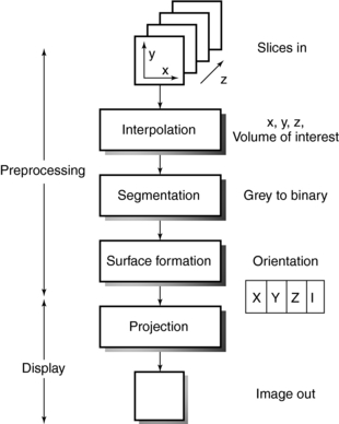
The applications of three-dimensional (3D) imaging are rapidly increasing (Calhoun et al, 1999; Cody, 2002; Dalrymple et al, 2005; Fishman et al, 2006; Logan, 2001; Udupa, 1999; Udupa and Herman, 2000). 3D imaging uses 3D surface and volumetric reconstruction. The algorithms for 3D imaging are based on those used in computer graphics and visual perception science. An algorithm for surface display (Fig. 6-16) is based on at least two processes, preprocessing and display, and consists of the following operations: interpolation, segmentation, surface formation, and projection (Cody, 2002; Udupa and Herman, 2000). 3D algorithms allow the user to “interactively visualize, manipulate, and measure large 3D objects on general purpose workstations” (Dalrymple et al, 2005; Fishman et al, 2006; Udupa and Herman, 2000).
REFERENCES
Berland, LL. Practical CT: technology and techniques. New York: Raven Press, 1987.
Bracewell, R. The Fourier transform,. Sci Am. 1989;260:86–95.
Brooks, RA, Di Chiro, G. Principles of computer assisted tomography (CAT) in radiographic and radioisotopic imaging,. Phys Med Biol. 1976;21:689–732.
Bruening, R, Flohr, T. Protocols for multislice CT—4 and 16 row applications. New York: Springer Verlag, 2003.
Calhoun, PS, et al. Three-dimensional volume rendering of spiral CT data: theory and method,. Radiographics. 1999;19:745–764.
Chen, L, et al. General surface reconstruction for cone beam multislice spiral computed tomography,. Med Phys. 2003;30:2804–2812.
Cody, DD. AAPM/RSNA physics tutorial for residents: topics in CT. Image processing in CT,. Radiographics. 2002;22:1255–1268.
Curry, TS, III., et al. Christensen’s physics of diagnostic radiology, 4. Philadelphia: Lea & Febiger, 1990.
Dalrymple, NC, et al. Introduction to the language of three-dimensional imaging with multidetector CT,. Radiographics. 2005;25:1409–1428.
Fishman, EK, et al. Volume rendering versus maximum intensity projection in CT angiography: what works best, when, and why,. Radiographics. 2006;26:905–922.
Flohr, TG, et al. Multi-detector row CT systems and image reconstruction techniques,. Radiology. 2005;235:756–773.
Gibson C, ed. The Facts on File dictionary of mathematics. New York: Facts on File, 1981.
Gordon, R, Herman, GT. Three-dimensional reconstruction from projections: a review of algorithms,. Int Rev Cytol. 1974;38:111–123.
Hein, I, et al. Feldkamp-based cone beam reconstruction for gantry-tilted helical multislice CT,. Med Phys. 2003;30:3233–3242.
Hounsfield GH: A method of and apparatus for examination of a body by radiation such as x or gamma radiation, London, British Patent Office, Patent No. 1283915, 1972.
Huang, HK. PACS: basic principles and applications. New York: Wiley-Liss, 1999.
Kalender, WA. Computed tomography: fundamentals, system technology, image quality, applications. Erlangen: GWA, 2005.
Knuth, DE. Algorithms,. Sci Am. 1977;236:63–80.
Kuhl, DE, Edwards, RQ. Image separation radioisotope scanning,. Radiology. 1963;80:653–661.
Logan, L. Seeing the future in three dimensions,. Radiol Technol. 2001;15:483–487.
Oldendorf, WH. Isolated flying spot detection radiodensity discontinuities displaying the internal structural pattern of a complex object,. IEEE Trans Biomed Eng BME. 1961;8:68–72.
Parker, JA. Image reconstruction in radiology. Boca Raton, Fla: CRC Press, 1991.
Parker, DL, Stanley, JH. Glossary. In: Newton TH, Potts DG, eds. Glossary Radiology of the skull and brain: technical aspects of computed tomography. St Louis: Mosby, 1981.
Ramachandran, GN, Lakshminarayanan, AV. Three-dimensional reconstructions from radiographs and electron micrographs: application of convolution instead of Fourier transforms,. Proc Natl Acad Sci U S A. 1971;68:2236–2240.
Seeram, E. Computed tomography technology. Philadelphia: WB Saunders, 2001.
Shepp, LA, Logan, BF. The Fourier reconstruction of a head section,. IEEE Trans Nucl Sci. 1974;21:21–43.
Udupa, JK. Three-dimensional visualization and analysis methodologies: a current perspective,. Radiographics. 1999;19:783–803.
Udupa, JK, Herman, GT. 3D imaging in medicine. Boca Raton: CRC Press, 2000.
BIBLIOGRAPHY
Cho, ZH, Ahn, IS. Computer algorithms for the tomographic image reconstruction with x-ray transmission scans,. Comput Biomed Res. 1975;8:8–25.
Fishman, EK, et al. Three-dimensional imaging,. Radiology. 1991;181:321–337.
Gabor, HT. Image reconstruction from projections. New York: Academic Press, 1980.
Kalender, WA, et al. Single-breath-hold spiral volumetric CT by continuous patient translation and scanner rotation,. Radiology. 1989;173:414–419.
Strong, AB, et al. Applications of three-dimensional display techniques in medical imaging,. J Biomed Eng. 1990;12:233–238.
*A line integral is the integral (summation of values that are infinitesimally close to each other multiplied by the infinitesimal distance separating the values) of a two-dimensional or three-dimensional object along the point of a line (Parker and Stanley, 1981).