Chapter 11 Physical principles of Doppler ultrasound
INTRODUCTION
This chapter provides the basic introduction to the physical principles and application of Doppler ultrasound in practice. The application of Doppler in ultrasound was first introduced in the 1980s and since then this technique has expanded in all specialist fields of practical ultrasonography.
A Doppler ultrasound is a non-invasive test that can be used to investigate movement and particularly evaluate blood flow in arteries and veins. It can also be used to provide information regarding the perfusion of blood flow in an organ or within an area of interest. A more recent application is the investigation of tissue wall motion when evaluating the heart (see Chapter 14 on New technology).
Doppler ultrasound can be used to diagnose many conditions, including:
THE DOPPLER PRINCIPLE
The Doppler principle is named after the mathematician and physicist Christian Johann Doppler who first described this effect in 1842 by studying light from stars. He demonstrated that the colored appearance of moving stars was caused by their motion relative to the earth. This relative motion resulted in either a red shift or blue shift in the light’s frequency. This shift in observed frequencies of waves from moving sources is known as the Doppler effect and applies to sound waves as well as light waves.
The Doppler Effect
An everyday example which demonstrates the Doppler effect is highlighted in Figure 11.1. We are all aware that the pitch of an ambulance siren changes as we stop and listen to it as it drives by. The frequency that reaches you is higher as the ambulance approaches and lower as the ambulance passes by. This is a consequence of the Doppler effect.
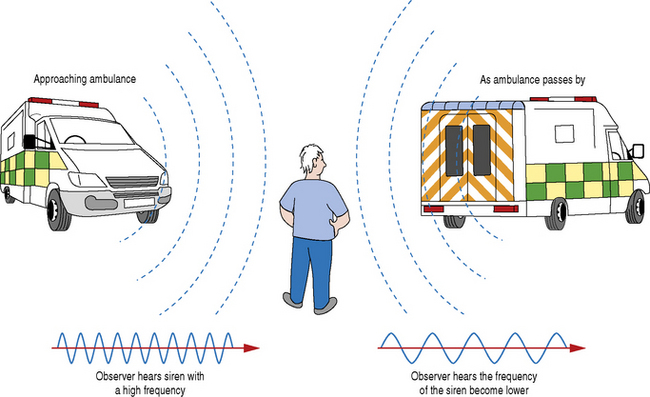
Fig. 11.1 The consequence of the Doppler effect on the relative emitted frequency of an ambulance siren as it drives by. The frequency of the approaching ambulance siren appears higher compared to the frequency of the siren as the ambulance passes by which appears lower
What is happening is that the sound waves are compressed when an object producing sound is moving in the same direction as the waves. The listener (observer) therefore receives shorter wavelengths. However, when the source of sound has passed the listener, the waves are now moving in the opposite direction (away from the listener), the wavelength becomes longer and the listener therefore hears a change in frequency.
This Doppler effect is utilized in ultrasound applications to detect blood flow by analyzing the relative frequency shifts of the received echoes brought about by the movement of red blood cells.
THE DOPPLER EFFECT APPLIED TO DIAGNOSTIC ULTRASOUND
The Doppler effect in diagnostic imaging can be used to study blood flow, for example, and provides the operator with three pieces of information to determine:
The transducer acts as both a transmitter and receiver of Doppler ultrasound. When using Doppler to investigate blood flow in the body, the returning backscattered echoes from blood are detected by the transducer. These backscattered signals (Fr) are then processed by the machine to detect any frequency shifts by comparing these signals to the transmitted Doppler signals (Ft). The frequency shift detected will depend on two factors, namely the magnitude and direction of blood flow (see Fig. 11.2).
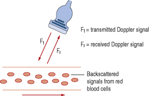
Fig. 11.2 An ultrasound transducer interrogating a blood vessel. Transmitting a Doppler signal with frequency Ft and receiving the backscattered signals from the red blood cells within the vessel at a frequency Fr
Let us consider a simple arrangement as seen in Figure 11.3. The transducer transmits a Doppler signal with frequency Ft. The transmitted Doppler signal interrogates a blood vessel and the transducer receives the backscattered signals from the red blood cells within the vessel at a frequency Fr. The Doppler frequency shift (Fd) can be calculated by subtracting the transmitted signal Ft from the received signal Fr.
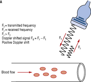
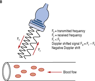
Fig. 11.3 Demonstrating the resulting Doppler shifted signals for a) blood flow moving towards the transducer; b) blood flow moving away from the transducer
Blood flow moving towards the transducer produces positive Doppler shifted signals and conversely blood flow moving away from the transducer produces negative Doppler shifted signals. Figure 11.3 illustrates the change in the received backscattered signals and the resulting Doppler shifts for blood moving towards and away from the transducer.
In Figure 11.3a the relative direction of the blood flow with respect to the Doppler beam is towards the transducer. In this arrangement blood flow moving towards the transducer produces received signals (Fr) which have a higher frequency than the transmitted beam (Ft). The Doppler shifted signal (Fd) can be calculated by subtracting Ft from Fr and produces a positive Doppler shifted signal.
Conversely, Figure 11.3b illustrates blood flow which is moving away from the Doppler beam and the transducer. In this arrangement blood flow moving away from the transducer produces received signals (Fr) which have a lower frequency than the transmitted beam (Ft). This time the Doppler shifted frequencies (Fr − Ft) produces a negative Doppler shifted signal.
When there is no flow or movement detected then the transmitted frequency (Ft) is equal to the received frequency (Fr). Therefore Fr = Ft and Fd = Fr − Ft = 0, resulting in no Doppler shifted signals.
It is important to appreciate that the amplitude of the backscattered echoes from blood is much weaker than those from soft tissue and organ interfaces which are used to build up our B-mode anatomical images. The amplitude of the backscattered signal from blood can be smaller by a factor of between 100 and 1000. Therefore highly sensitive and sophisticated hardware and processing software is required to ensure that these signals can be detected and processed.
THE DOPPLER EQUATION
The Doppler equation shows the mathematical relationship between the detected Doppler shifted signal (Fd) and the blood flow velocity (V):
Ft = transmitted Doppler frequency
c = the propagation speed of ultrasound in soft tissue (1540 ms−1)
V = velocity of the moving blood
θ = the angle between the Doppler ultrasound beam and the direction of blood flow
The number 2 is a constant indicating that the Doppler beam must travel to the moving target and then back to the transducer.
Equation 1: The Doppler equation.
Relationship between Doppler Shifted Signal (Fd) and Blood Flow Velocity (V)
The Doppler equation (Equation 1) demonstrates that there is a relationship between the Doppler shifted signal (Fd) and the blood flow velocity (V). The Doppler shifted signal (Fd) is directly proportional to the blood flow velocity (V), which means greater flow velocities create larger Doppler shifted signals and conversely lower flow velocities generate smaller Doppler shifted signals. If we can detect and measure the value of Fd then the Doppler equation can be rearranged (see Equation 2) to calculate blood flow velocities (V) which can be processed and displayed.
Equation 2: Doppler equation rearranged to calculate blood flow velocities (V).
Significance of the Doppler Angle (θ)
Ultrasound machines are able to calculate Doppler shifted frequencies over a wide range of angles and it is important that an operator understands the significance of the angle of insonation (θ) between the Doppler beam and the direction of blood flow in vessels. Figure 11.4 graphically shows how the Doppler shifted signal changes as the Doppler beam angle changes.
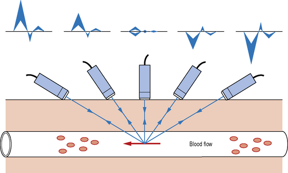
Fig. 11.4 Graphically demonstrating the relationship between the Doppler shifted frequency with respect to the angle of the insonating Doppler beam
When the Doppler beam is pointing towards the direction of blood flow a positive Doppler shifted signal is observed, but once the Doppler beam is pointed away from the direction of blood flow a negative Doppler shifted signal is seen. The smaller the angle between the Doppler beam and blood vessel, the larger the Doppler shifted signal. Very small signals are produced as the Doppler beam angle approaches a 90° angle.
Table 11.1 shows the relationship between the angle of the Doppler beam (θ) and the value of cosθ. The value of cosθ varies with the angle from 0 to 1. When θ = 0°, cosθ = 1 and when θ = 90°, cosθ = 0.
Table 11.1 Variation of the value of cosθ over a range of angles of insonation. Maximum value of cosθ corresponds to a Doppler beam angle of 0°.
| ANGLE θ | VALUE OF COSθ |
|---|---|
| 0 | 1 |
| 30 | 0.87 |
| 45 | 0.71 |
| 60 | 0.5 |
| 75 | 0.26 |
| 90 | 0 |
For a constant flow velocity (V), the maximum value of cosθ and therefore the highest value of the Doppler shifted signal (Fd) is at an angle of 0°. This corresponds to a Doppler beam which is parallel with the vessel, which can rarely be achieved in practice.
Theoretically, when θ = 90° this means the blood flow is perpendicular to the Doppler beam, cosθ = 0 and no Doppler shifted signals will register.
In practice, when taking measurements of blood flow, a Doppler beam angle of between 30 and 60° is important to ensure reliable Doppler shifted signals. Avoid using angles greater than 60° and remember no Doppler shifted signals are generated at 90°.
Greater flow velocities and smaller angles produce larger Doppler shifted frequencies, but not stronger Doppler shift signals.
Typical Doppler Shifted Signals for Blood Flow
Ultrasound machines transmit high-frequency sound waves which lie in the megahertz range, typically between 2 MHz and 20 MHz. Substituting typical physiological blood flow velocities into the Doppler equation gives Doppler shifted signals which lie within the audible range. That is, the range of frequencies that the human ear can hear. A healthy young human can usually hear from 20 cycles per second to around 20 000 cycles per second (20 Hz to 20 kHz).
Let us calculate a typical Doppler signal frequency for blood moving at 0.5 ms−1 which is illustrated in Figure 11.5. Transmitted frequency (Ft) is 4 MHz, θ = 60° and c (the propagation speed of ultrasound) is assumed constant at 1540 ms−1.
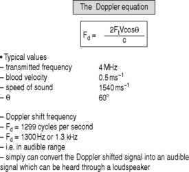
Fig. 11.5 Illustrates the calculated Doppler shifted signal using the Doppler equation for blood flow moving at 50 cm/s for a Doppler beam operating at 4 MHz positioned with an insonation angle of 60°
Using the Doppler equation (Equation 1) we calculate the Doppler shifted frequency to be 1299 cycles per second, about 1300 Hz or abbreviated to 1.3 kHz.
These generated Doppler shifted signals can simply be converted into an audible signal which can be heard and monitored through a loudspeaker.
TYPES OF DOPPLER INSTRUMENTATION IN DIAGNOSTIC IMAGING
There are a number of types of Doppler instrumentation used in ultrasound which include:
Doppler techniques applied to diagnostic ultrasound can be characterized as either being non-imaging or imaging. Non-imaging techniques typically use small or handheld units, and use continuous wave (CW) Doppler. The main purpose of these simple CW units is to either identify and/or monitor blood flow. Two examples of clinical examinations include fetal heart monitors in obstetrics and peripheral blood flow assessment in vascular practice.
Imaging Doppler techniques such as color and spectral PW Doppler are always used with B-mode imaging where the gray scale anatomical image is used to identify blood vessels and areas for blood flow evaluation. These techniques require more sophisticated processing than CW devices.
Continuous Wave Doppler Devices
Continuous wave (CW) Doppler devices are the simplest of Doppler instruments and typically consist of a handheld unit with an integrated speaker which is connected to a pencil probe transducer (Fig. 11.6).
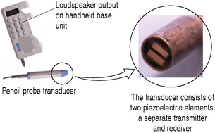
Fig. 11.6 A simple CW Doppler device illustrating the two piezoelectric elements at the tip of the pencil probe transducer: one acting as a continuous transmitter, the other acting as a continuous receiver
The transducer consists of two piezoelectric elements: one element acts as a continuous transmitter (Ft) and the other acts as a continuous receiver (Fr).
These two elements are set at an angle to each other so that the transmit and reception beams overlap one another, as illustrated in Figure 11.7. This crossover region is known as the active or sensitive area and is where Doppler signals can only be detected. Doppler shift signals (Fd) are detected by comparing the transmitted and received signals: Fd = Fr − Ft.
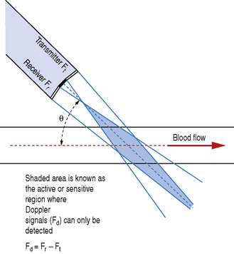
Fig. 11.7 Elements within the transducer are set at a fixed angle. Doppler signals only detected where the transmitter and receiver beams overlap
The frequency and angle between the two elements within the transducer are determined by the clinical application.
For example, using CW Doppler in obstetrics for fetal heart monitoring requires a sufficiently low-frequency Doppler signal to be able to penetrate to the required depth; typically 4 MHz is used. The angle and therefore active crossover region between the two elements is also set to correspond to the required depth of integration.
Contrast this with the assessment of the peripheral circulation in the legs. Here the CW Doppler device is required to detect blood flow in vessels which lie very close to the skin surface. So here a higher Doppler transmit frequency can be used, typically 8 MHz, and the angle between the two crystals within the probe is greater so that the crossover region corresponds to the required depth of only a couple of centimeters.
There are various CW Doppler devices available to detect blood flow. These range from simple inexpensive handheld Doppler units, where the Doppler signal is processed to provide an audible output, to more sophisticated devices which provide a visual display of the Doppler shifted blood flow patterns.
The main disadvantage of CW devices is that the transducer is sensitive to any blood flow within the crossover region. If more than one vessel is present in this crossover region then Doppler signals are obtained from more than one vessel at a time. Arteries and veins often lie adjacent to each other so in many cases CW devices will simultaneously detect arterial and venous flow signals. In addition, CW devices are unable to provide information on the depth from which the blood flow signals have returned and cannot measure blood flow velocity (V).
The advantages of CW Doppler devices are that they are small and cheap and are relatively easy to use with minimal training. Blood flow can be detected and monitored through a loudspeaker or blood flow patterns can be displayed graphically.
Table 11.2 summarizes the advantages and disadvantages of CW Doppler devices.
Table 11.2 Comparative advantages and disadvantages of CW Doppler.
| CW DOPPLER DEVICES | |
|---|---|
| ADVANTAGES | DISADVANTAGES |
| Small | Cannot distinguish multiple vessels within crossover region |
| Cheap – simple design | Cannot measure velocity |
| Relatively easy to use and to search for a vessel | Unable to provide information about depth |
| Can display blood flow patterns | |
Color Flow Imaging
Color flow imaging was first introduced in the mid 1980s and since then has extended the role of ultrasound as a diagnostic tool. It can quickly and effectively enable the operator to identify the presence and direction of blood flow in vessels and can highlight gross circulation anomalies within the anatomical B-mode image.
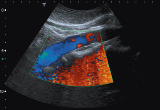
It is probably the first Doppler technique that an operator will utilize to investigate blood flow. Color flow imaging is always used in conjunction with B-mode imaging and once it is activated the operator is presented with a region of interest known as the ‘color box’ and vertical ‘color scale’ bar which are superimposed onto the B-mode image, as illustrated in Figure 11.8.
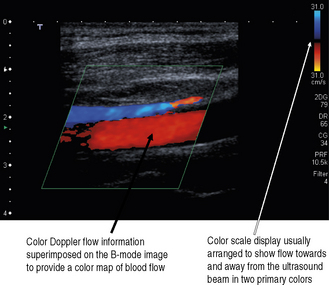
Fig. 11.8 B-mode image with color flow information superimposed. Note that color flow information is only mapped into the color box region. Vertical color scale bar present on the right-hand side of the display
Unlike CW Doppler devices, where continuous Doppler beams are generated and transmitted by the two separate elements within the transducer, color flow imaging uses small groups of elements to transmit and receive the Doppler signals. The Doppler signals consist of a series of short bursts or pulses of ultrasound similar to those used in B-mode imaging. To form the color flow image, additional Doppler ultrasound pulses are generated by the transducer which is typically three to four times longer than those used for B-mode imaging. The transducer elements are rapidly switched between B-mode and color flow imaging to give an impression of a combined simultaneous image, and this is often known as duplex imaging, duplex meaning ‘double’.
The position and size of this color box can be adjusted to the chosen area of interest by the operator to provide a visual color-coded display or map of blood flow.
The color box
The color image within the color box is made up of hundreds of scan lines which are each subdivided into small sample volumes as illustrated in Figure 11.9. Typically, there are hundreds of sample volumes per scan line, amounting to thousands of sample volumes within the color box.
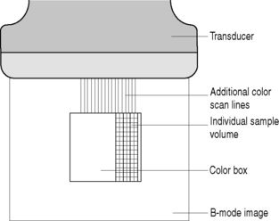
Fig. 11.9 The color flow box is made up of hundreds of scan lines. Each scan line consists of hundreds of small sample volumes which individually detect the backscattered Doppler ultrasound signals
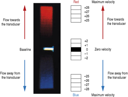
For each individual sample volume along each scan line, the average or mean Doppler shifted velocity is calculated. This mean Doppler shifted velocity, which can either be positive or negative, is assigned a color which is then mapped onto a color scale which consists of two primary colors. This is usually red for positive Doppler shifted signals (corresponding to blood flow traveling towards the transducer) and blue for negative Doppler shifted signals (corresponding to blood flow away from the transducer). This typical arrangement can be seen in Figure 11.8.
Once this directional information is processed, the sample volume is assigned a shade or hue depending on the calculated mean velocity.
The color flow information in the color box is made up by processing the information in each sample volume along each scan line in turn. In order to obtain a reliable estimation of the mean velocity in each sample volume, several (10 or more) pulse-echo sequences are required to produce each scan line of color flow information. This series of pulse-echo sequences is then repeated for the next adjacent scan line, and so on, as is the case for B-mode imaging.
A consequence of this multi pulse-echo technique is that it takes more time to collect and process the information required for color flow imaging than it does for standard B-mode imaging. As a result, color flow images tend to have lower frame rates than those used in B-mode.
Color scale
The color scale is represented as a vertical color bar and normally sits to the side of the B-mode image (see Fig. 11.8). Closer inspection of the color bar shows that it consists of two primary colors with each primary color subdivided into different shades or hues.
Just as in B-mode imaging, where returning echo amplitudes are assigned a varying level of gray to form the B-mode image (higher echo amplitudes are assigned brighter levels of gray and low amplitude echoes are assigned darker shades of gray), in color flow imaging similarly higher calculated mean flow velocities are assigned varying hues of red and blue. The higher the velocity, the brighter the shade or hue assigned.
Figure 11.10 illustrates a typical color scale bar used. As you can see, it consists of a vertical color bar which is split from the center into two primary colors. The center of a standard color bar scale represents zero or no flow. In this case, blood flow towards the transducer will be labeled red and blood flow away from the transducer is labeled blue. However, in most equipment this color bar scale can be changed, if required, by the operator.
Significance of angle
With any Doppler technique, angle is important. The appearance of the color flow image is very much dependent on the operator to obtain a sufficient angle between the Doppler ultrasound beam and the vessel.
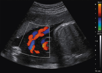
Curvilinear and phased array transducers have a radiating pattern of ultrasound beams that can produce complex color flow images, depending on the orientation of the arteries and veins with respect to the Doppler beam. This can be seen in Figure 11.11 which presents a color flow image of an umbilical cord.
Many peripheral vessels run parallel to the face of a linear transducer and perpendicular to the Doppler beam. If the angle of the Doppler beam with respect to the vessel is at 90°, little or no Doppler signal will be detected, as seen in Figure 11.12. When using a linear array transducer the operator is able to overcome this problem by electronically steering the Doppler beam. This is performed by altering the angle of the color box, as illustrated in Figure 11.13. The objective is toobtain a sufficiently small angle between the Doppler beam and blood vessel to provide reliable Doppler signals.
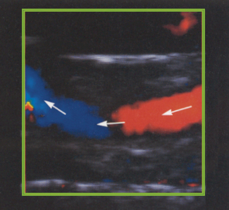
Fig. 11.12 Color flow imaging demonstrating that no Doppler signal is registered when the vessel is at 90° with the Doppler beam
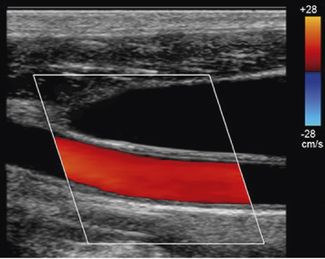
Fig. 11.13 Color flow image of the common carotid artery with a steered color box to obtain sufficient angles for reliable Doppler signals
In practice, an experienced operator alters the scanning approach and steers the Doppler beam to obtain good angles between the Doppler beam and vessel to avoid unambiguous color flow images.
Aliasing
Aliasing occurs with all pulsed wave Doppler instruments because they employ a sampling method to build up the Doppler shifted signals.
The color flow information is not built up continuously, as is the case with CW Doppler devices, but is formed from a series of Doppler ultrasound pulses which are transmitted at a given rate known as the sampling frequency.
In order to measure the many Doppler shifted frequencies present in typical blood flow patterns, thousands of pulses are sent along each scan line in turn. These sampled pulses are used to build up the Doppler shifted signal and in order to accurately build the Doppler shifted signal there must be an adequate number of samples per second.
Aliasing is the incorrect estimation of Doppler shifted signals due to undersampling which causes a false lower Doppler shifted frequency signal to appear in the sampled signal. Figure 11.14 shows an undersampled signal and an adequately sampled signal of a simple sine wave.
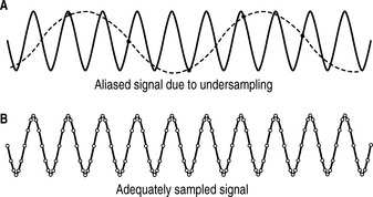
In Figure 11.14a the undersampled signal appears to have a lower frequency than the actual signal – two cycles instead of ten cycles.
Increasing the sampling frequency as demonstrated in Figure 11.14b increases the number of data points acquired in a given time period. A rapid sampling frequency provides a better representation of the original signal than a slower sampling frequency.
The effect of aliasing can be seen when watching films where wagon wheels can appear to be going backwards instead of forwards due to the low frame rate of the film causing misinterpretation of the movement of the wheel spokes. The true velocity and correct direction of the wheel is only seen if the film’s frame rate is rapid enough.
Significance of pulse repetition frequency
The frequency, i.e. sampling rate, at which these pulses can be sent is determined by the system’s pulse repetition frequency (PRF) which can be adjusted through the color scale control button. Increasing the color scale increases the system’s PRF and, conversely, reducing the color scale will reduce the system’s PRF.
There is an upper limit to the system’s PRF, i.e. color scale, which is restricted to the time the system has to wait to receive all the returning echoes along each scan line before sending another. This is linked to the maximum Doppler shifted signals (Fd) that can be detected. The maximum Doppler shifted signal Fd that can be measured is restricted, and is equal to half the pulse repetition frequency of the system, which is mathematically represented below:

This condition is known as the Nyquist limit. If the Nyquist limit is exceeded then aliasing will occur. When aliasing occurs, the displayed colors ‘wrap around’ the color scale bar and the colors change from the maximum color in one direction to the maximum in the opposite direction.
Figure 11.15a illustrates color aliasing which is caused when the color scale is set too low. The Doppler signals are undersampled at a PRF = 12.5 kHz which corresponds to a maximum color scale velocity of 13.9 cm/s. In this example, color flow changes from BLUE to RED are observed within the vessel. Increasing the color scale increases the PRF, from 12.5 kHz to 14 kHz, which is sufficient enough to eliminate aliasing within the image, as demonstrated in Figure 11.15b.
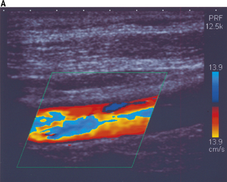
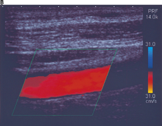
Fig. 11.15 a) The color scale is set too low, resulting in aliasing of the color Doppler signal. The Doppler signals are undersampled at a PRF = 12.5 kHz. b) The color scale and PRF are increased to ensure that the Doppler signals are adequately sampled, resulting in the elimination of aliasing. This is achieved at a higher PRF of 14 kHz
Significance of depth
A relationship exists between the maximum velocity of blood that can be detected and the maximum depth at which a vessel is investigated. As the depth of investigation increases, the journey time of the pulse to and from the reflector is increased; this in turn reduces the system’s PRF. This reduction in the system’s PRF reduces the maximum Doppler shifted signal (Fd) that can be displayed before aliasing occurs. The result is that the maximum Doppler shifted signals (Fd) which can be measured decrease with depth.
Power Doppler
Power Doppler is also referred to as energy Doppler, amplitude Doppler and Doppler angiography. It is a color flow imaging technique that maps the magnitude, i.e. power, of the backscattered Doppler signal rather than the Doppler shifted flow velocities. The instantaneous signal strength contained in the Doppler signal is calculated and superimposed onto the B-mode image as illustrated in Figure 11.16. Its effect is to provide a map of areas of perfusion, by displaying the amplitude of red blood cells in an area.
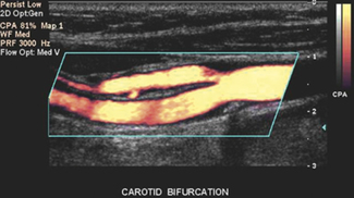
Power Doppler does not display the relative velocity and direction of blood flow as is the case with color flow imaging. Power Doppler uses a single color scale and maps increasing signal strengths to increased luminosity. It is often used in conjunction with frame averaging to increase sensitivity to low flows and velocities.
Power Doppler has several advantages over color flow imaging which include:
Spectral or Pulse Wave Doppler
Spectral Doppler, also referred to as pulsed wave (PW) Doppler, is combined with B-mode and color flow imaging techniques and allows for the assessment and evaluation of the blood flow over a very small region known as the sample volume. This technique is known as range gating.
When spectral Doppler is initially instigated, a single Doppler beam axis is superimposed onto the B-mode and color flow image as illustrated in Figure 11.17. The size and position of the sample volume can be adjusted anywhere along the axis of the Doppler beam and this information is displayed on the monitor. The position of the sample volume determines where along the Doppler beam blood flow velocities are to be investigated. The size of the sample volume determines how much of the vessel is examined. For arterial examinations, the sample volume is positioned in the center of the vessel, and the size of the sample volume is set to be approximately one half to one third of the diameter of the vessel.
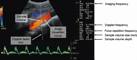
Fig. 11.17 Illustration of the on-screen components when spectral Doppler is activated. Highlighting the Doppler beam axis, the sample volume, and angle correction cursor. The size and position of the sample volume is always displayed on screen
When the sample volume has been correctly positioned over a point of interest then the spectral Doppler display is activated to provide blood flow velocity information.
The Doppler beam itself can be maneuvered over the B-mode image and follows the path of the B-mode imaging scan lines for a sector array transducer, as depicted in Figure 11.17. When linear array transducers are used, the Doppler beam can be steered, which enables the operator to achieve the necessary angle between the Doppler beam and blood vessel under investigation. An example of this is shown in Figure 11.18.
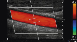
Fig. 11.18 An example of a linear array transducer electronically steering both the color and spectral Doppler beams to obtain a sufficient angle between the Doppler beam and blood vessel for reliable Doppler assessment
The angle correction cursor which is located at the center of the sample volume is used to estimate the angle of insonation between vessel and Doppler beam and should be adjusted to align with the direction of blood flow in the vessel to calculate absolute flow velocities from the detected Doppler shifted signals.
By angle correcting, the operator provides the ultrasound system with the actual value of θ in the Doppler equation. Once θ is known, the Doppler equation can be used to calculate actual blood flow velocities. Accurate and reliable spectral Doppler flow velocities are achieved for angles of θ, between the Doppler beam and the direction of blood flow, which are no greater than 60°.
Color flow imaging which maps blood flow over a much larger area is used in conjunction with spectral Doppler, highlighting areas of disturbed or turbulent blood flow for spectral Doppler assessment.
Spectral Doppler, combined with real-time B-mode and color flow imaging, is known as triplex imaging. When triplex imaging is used by the operator, data collecting and processing is shared between all three modes. This reduces the overall imaging frame rate and Doppler sampling frequency, which in turn restricts the range over which blood flow velocities can be measured.
Optimum spectral Doppler assessments are achieved when B-mode and color flow imaging modes are temporarily frozen which allows more time to be employed for rapid spectral Doppler processing.
Generation of spectral PW Doppler signals
Spectral Doppler is similar to color flow imaging in the way that it utilizes a sampling technique to build up the spectral Doppler shifted signals. As is the case for B-mode imaging, a small group of elements within the transducer acts as both a transmitter and receiver of Doppler ultrasound, transmitting regular short bursts of spectral Doppler signals from which received Doppler shifted signals are processed. However, spectral Doppler only sends out one beam, unlike color Doppler which requires many adjacent beams to form the color flow image. The pulses generated for spectral Doppler differ from those used for B-mode imaging and tend to be longer, typically 6–10 cycles in length.
Processing and displaying the PW Doppler signal
Spectral Doppler provides more detailed information of blood flow than color flow imaging and is able to map the variation and distribution of blood flow velocities over the cardiac cycle. The spectral Doppler signal contains all this information.
Doppler signals are processed using spectral analysis to provide a more meaningful and useful way to represent the Doppler velocity information visually. Spectral analysis breaks down the Doppler signals received within the sample volume into its range of frequency components, which are translated into a range of flow velocities. The process of spectral analysis can be thought of as being similar to using a prism to split visible light into its separate components, i.e. its color spectrum, as seen in Figure 11.19.

Fig. 11.19 A prism splitting light into its individual components is similar to the process employed by spectral analysis
Figure 11.20 shows a typical spectral analysis trace for a femoral artery, with time along the horizontal axis and flow velocities (calculated from the Doppler shifted signals) along the vertical axis. The vertical axis is divided into two so that both positive and negative Doppler shifted signals can be displayed. The baseline relates to zero flow. Both the velocity scale and baseline can be adjusted by the operator to ensure that spectral waveforms are optimally displayed.
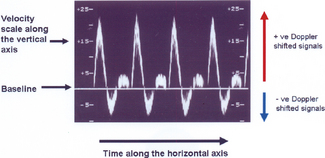
Fig. 11.20 Spectral waveform of a femoral artery displaying time along the horizontal axis and flow velocities along the vertical axis
The third axis of the spectral trace corresponds to the backscattered power of the Doppler shifted signal at each velocity. This is simply displayed as brightness which is illustrated in Figure 11.21.
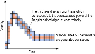
Fig. 11.21 A spectral analysis trace displaying the variation of velocities over the cardiac cycle. The brightness corresponds to the backscattered power of the Doppler shifted signal at each velocity
Spectral analysis is performed by the ultrasound machine’s on-board computer using a mathematical technique known as a fast Fourier transform (FFT) and produces between 100–200 lines of processed data every second. PW Doppler systems are able to process information fast enough to produce real-time spectral Doppler waveforms and, as a consequence of this, rapid processing is said to have good temporal resolution.
Aliasing
Because spectral Doppler uses a sampling technique to interrogate and build up information about the blood flow velocities, it is subject to aliasing. As discussed under Color Flow Imaging, aliasing is governed by the system’s Doppler PRF which can be adjusted through the spectral Doppler ‘scale’ control. The maximum velocity that can be measured is directly proportional to half the value of the PRF. The higher the pulse repetition frequency of the Doppler pulses, the higher the Doppler shifted velocity that can be measured. The PRF is also linked to the position (i.e. the depth) of the sample volume. The deeper the sample volume is placed within the B-mode image, the lower the value of the PRF due to time constraints, i.e. the system has to wait longer to receive the reflected Doppler pulses from a sample volume which is placed deep within the image rather than one which is positioned close to the transducer. The relationship between PRF, the maximum measurable velocity, and the depth of the sample volume are summarized in Table 11.3.
Table 11.3 Demonstrating the relationship between PRF, maximum measurable velocity, and depth of sample volume.
| ACTION | CONSEQUENCE | |
|---|---|---|
| As PRF increases | Maximum measurable velocity increases | |
| As PRF decreases | Maximum measurable velocity decreases | |
| As the depth of sample volume increases | PRF decreases | Maximum measurable velocity decreases |
| As the depth of sample volume decreases | PRF increases | Maximum measurable velocity increases |
The effects of aliasing are demonstrated in Figure 11.22 and cannot always be eliminated, as it is not always possible to have the PRF significantly higher than the Doppler shifted signal. However, these effects can be minimized by adjusting the following controls:
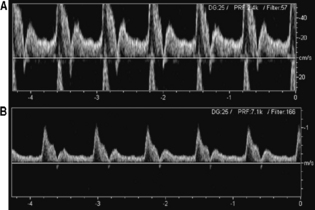
Fig. 11.22 Example of aliasing and correction of the aliasing. a) Waveforms with aliasing wrap around the velocity scale resulting in the peaks being displayed below the baseline. b) Aliasing avoided with the same spectral waveform achieved by increasing the pulse repetition frequency, i.e. increasing the velocity scale
Advantages and disadvantages of spectral Doppler
Advantages
Disadvantages
Table 11.4 summarizes and compares these three Doppler modes.
Table 11.4 Comparison and summary of Doppler flow imaging modes.
| DOPPLER FLOW IMAGING MODE | MAIN ADVANTAGES AND DISADVANTAGES |
|---|---|
| Color flow imaging | |
| Power Doppler | |
| Spectral Doppler |
DOPPLER ARTIFACTS
Aliasing
Aliasing is the most common Doppler artifact and occurs with all pulsed wave Doppler instruments because they employ a sampling method to build up the Doppler shifted signals. Aliasing is the incorrect estimation of Doppler shifted signals due to undersampling. When aliasing occurs, the displayed Doppler shifted signals ‘wrap around’ the Doppler velocity scale and the Doppler shifted signals change from the maximum velocity in one direction to the maximum in the opposite direction. Figures 11.15 and 11.22 demonstrate the effects of aliasing upon the color and spectral Doppler imaging displays.
Doppler Mirror Image
This type of artifact can be seen in both spectral Doppler and color flow imaging.
This mirror artifact can be seen in spectral Doppler traces where there is electronic duplication of spectral information being displayed below the zero baseline, as seen in Figure 11.23. It commonly results from the Doppler receiver gain being set too high.
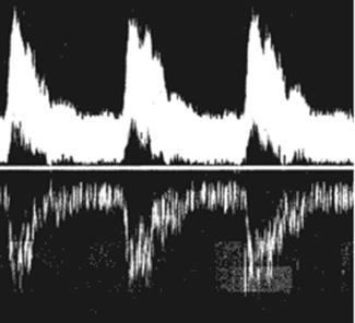
Fig. 11.23 Demonstrating spectral Doppler mirror artifact due to the receiver gain being set too high
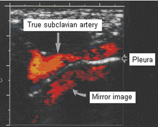
Color images can also produce mirror artifacts and can normally be seen where a vessel lies above a strong reflecting surface. Figure 11.24 shows a mirror image of the subclavian artery produced by multiple reflections from the pleura above the lung, where there is a soft-tissue/air boundary present, causing strong reflections.
Flash artifact
Both color flow and power Doppler imaging use filters to suppress signals arising from stationary or near stationary tissue. However, large movements of tissues brought about by heavy respiration or rapid transducer movement, for example, can cause significant flashes of color across large areas within the color flow image. Some machines have motion suppression algorithms to reduce this flash artifact. This is illustrated in Figure 11.25.