Using Statistics to Examine Relationships
Correlational analyses identify relationships between or among variables. In addition, the analysis may be used to clarify the relationships among theoretical concepts or assist in identifying causal relationships, which can then be tested by inferential analysis. The researcher should obtain all data for the analysis from a single population from which values are available on all variables to be examined. Data measured at the interval level will provide the best information on the nature of the relationship (i.e., if it is positive or negative). However, analysis procedures are available for most levels of measurement. To prepare for correlational analysis, the researcher plans data collection strategies to maximize the possibility of obtaining the full range of possible values on each variable.
This chapter discusses the use of scatter diagrams before correlational analysis, bipolar correlational analysis, testing the significance of a correlational coefficient, the correlational matrix, spurious correlations, the role of correlation in understanding causality, and multivariate correlational procedures, including factor analysis.
SCATTER DIAGRAMS
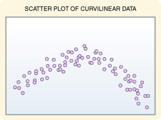
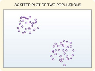
Scatter diagrams provide useful preliminary information about the nature of the relationship between variables. The researcher should develop and examine scatter diagrams before performing correlational analysis. Scatter diagrams may be useful for selecting appropriate correlational procedures, but most correlational procedures are useful for examining linear relationships only. A scatter plot can easily identify nonlinear relationships; if the data are nonlinear, the researcher should select other approaches to analysis (Figure 20-1). In addition, in some cases, data for correlational analysis have been obtained from two distinct populations. If the populations have different values for the variables of interest, the researcher will obtain inaccurate information on relationships among the variables. Differences in values from distinctly different populations are clearly visible on a scatter plot, thus allowing accurate interpretation of correlational results (Figure 20-2).
BIVARIATE CORRELATIONAL ANALYSIS
Bivariate correlation measures the extent (strength and direction) of linear relationship between two variables and is performed on data collected from a single sample. Measures of the two variables to be examined must be available for each subject in the data set. Less commonly, data are obtained from two related subjects, such as blood lipid levels in father and son. The statistical analysis techniques used will depend on the type of data available. Correlational techniques are available for all levels of data: nominal (phi, contingency coefficient, Cramer’s V, and lambda), ordinal (gamma, Kendall’s tau, and Somers’ D), or interval and ratio (Pearson’s correlation). Many of the correlational techniques (gamma, Somers’ D, Kendall’s tau, contingency coefficient, phi, and Cramer’s V) are used in conjunction with contingency tables. Contingency tables are explained further in Chapter 22.
Correlational analysis provides two pieces of information about the data: the nature or direction of the linear relationship (positive or negative) between the two variables and the magnitude (or strength) of the linear relationship. The outcomes of correlational analysis are symmetrical rather than asymmetrical. Symmetrical means that the direction of the linear relationship cannot be determined from the analysis. One cannot say from the analysis that variable A causes variable B.
In a positive linear relationship, the scores being correlated vary together (in the same direction). When one score is high, the other score tends to be high; when one score is low, the other score tends to be low. In a negative linear relationship, when one score is high, the other score tends to be low (for example, height and weight). A negative linear relationship is sometimes referred to as an inverse linear relationship (for example, the number of courses taken at one time and GPA). You can plot these linear relationships as a straight line on a graph. Sometimes, the outcome is not linear, but curvilinear, in which case a linear relationship plot will appear as a curved line rather than a straight one. (At first the relationship is positive, then it becomes negative. An example is memory and age.) Analyses designed to test for linear relationships, such as Pearson’s correlation, cannot detect a curvilinear relationship.
Pearson’s Product-Moment Correlation Coefficient
Pearson’s correlation was the first of the correlation measures developed and is the most commonly used. All other correlation measures have been developed from Pearson’s equation and are adaptations designed to control for violation of the assumptions that must be met to use Pearson’s equation. These assumptions are as follows:
1. Interval measurement of both variables (e.g., years of education and income)
2. Normal distribution of at least one variable
Data that are homoscedastic are evenly dispersed both above and below the regression line, which indicates a linear relationship on a scatter diagram (plot). Homoscedasticity reflects equal variance of both variables. In other words, for every value of x, the distribution of y scores should have equal variability. A regression line is the line that best represents the values of the raw scores plotted on a scatter diagram.
Calculation
Numerous formulas can be used to compute Pearson’s r. With small samples, Pearson’s r can be generated fairly easily with a calculator by using the following formula:
where

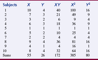
An example demonstrates the calculation of Pearson’s r. Correlation between the two variables of functioning and coping was calculated. The functional variable (variable X) was operationalized by using Karnofsky’s scale, and a family coping tool was used to operationalize coping. Karnofsky’s scale ranges from 1 to 10; 1 is normal function, and 10 is moribund (fatal processes progressing rapidly). Nursing diagnosis terminology was used to develop the family coping tool (variable Y); scores ranged from 1 to 4, with 1 being effective family coping; 2, ineffective family coping, potential for growth; 3, ineffective family coping, compromised; and 4, ineffective family coping, disabling. Table 20-1 presents the data for these two variables in 10 subjects. Usually, correlations are conducted on larger samples; this example serves only to demonstrate the process of calculating Pearson’s r:
Interpretation of Results
The outcome of the Pearson product-moment correlation analysis is an r value of between –1 and +1. This r value indicates the degree of linear relationship between the two variables. A score of zero indicates no linear relationship.
A value of –1 indicates a perfect negative (inverse) correlation. In a negative linear relationship, a high score on one variable is related to a low score on the other variable. A value of +1 indicates a perfect positive linear relationship. In a positive linear relationship, a high score on one variable is associated with a high score on the other variable. A positive correlation also exists when a low score on one variable is related to a low score on the other variable. A perfect positive or negative correlation is almost nonexistent between variables. As the negative or positive values of r approach zero, the strength of the linear relationship decreases. Traditionally, an r value of < 0.03 is considered a weak linear relationship, 0.3 to 0.5 is a moderate linear relationship, and > 0.5 is a strong linear relationship. However, this interpretation depends to a great extent on the variables being examined and the situation within which they were observed. Therefore, as a researcher you will need to apply some judgment when interpreting the results. In the example provided, the r value was 0.907, which indicates a strong positive linear relationship between the Karnofsky scale and the family coping tool in this sample.
Nursing researchers have tended to disregard weak correlations. However, such tendencies create a serious possibility of ignoring a linear relationship that may have some meaning within nursing knowledge when examined in the context of other variables. This situation is similar to a type II error (failing to reject the null when it is false) and commonly occurs for three reasons. First, many nursing measurements are not powerful enough to detect fine discriminations, and some instruments may not detect extreme scores. In this case, the linear relationship may be stronger than indicated by the crude measures available. Second, correlational studies must have a wide range of variance for linear relationships to be detected. If the study scores are homogeneous or if the sample is small, linear relationships that exist in the population will not show up as clearly in the sample. Third, in many cases, bivariate analysis does not provide a clear picture of the dynamics in the situation. A number of variables can be linked through weak correlations, but together they provide increased insight into situations of interest. Therefore, although one should not overreact to small Pearson coefficients, the information must be recorded for future reference. If the linear relationship is intuitively important, one may have to plan better-designed studies and reexamine the linear relationship.
Testing the Significance of a Correlational Coefficient
To infer that the sample correlation coefficient applies to the population from which the sample was taken, statistical analysis must be performed to determine whether the coefficient is significantly different from zero (no correlation). In other words, we can test the hypothesis that the population Pearson correlation coefficient is 0. The test statistic used is the t, distributed according to the t distribution, with n – 2 degrees of freedom. The formula for calculating the t statistic follows. This formula was used to calculate the t value for the example where r = 0.907:

where
The statistical significance of the t obtained from the formula is determined by using the t distribution table in Appendix A. With a small sample, a very high correlation coefficient (r) can be nonsignificant. With a very large sample, the correlation coefficient can be statistically significant when the degree of association is too small to be clinically significant. Therefore, when judging the significance of the coefficient, you must consider both the size of the coefficient and the significance of the t-test. The t value calculated in the example was 6.09, and the df for the sample was 8. This t value was significant at the 0.001 level. If the p value of the t test is significant, then the r value is statistically significant. When reporting the results of a correlation coefficient, both the r value and the p value should be reported.
The r value also must be examined for clinical importance. To do this, square the r value (r2) to determine the percentage of variance explained by this relationship. The stronger the r value, the greater the variability that is explained for the two variables. If the r value is of at least moderate strength (r = 0.3) or high, then the percentage of variance explained is 9% or higher. If the percentage of variance explained is 9% or higher the relationship has potential clinical importance that the researcher must evaluate. Research reports would be strengthened by discussing the statistical significance and clinical importance of an r value (Grove, 2007).
When Pearson’s correlation coefficient is squared (r2), the resulting number is the percentage of variance explained by the linear relationship. This is also called the coefficient of determination. In the preceding computation based on data in Table 20-3, r = 0.907 and r2 = 0.822. In this case, the linear relationship explains 82% of the variability in the two scores. Except for perfect correlations, r2 will always be lower than r. This r value is very high. Results in most nursing studies will be much lower. r2 is important because it helps correct for sample size issues, for example when large sample sizes are more likely to result in significant correlations.
Correlational Matrix
A correlational matrix is obtained by performing bivariate correlational analysis on every pair of variables in the data set. Figure 20-3 shows the appearance of the matrix. On the matrix, the r value and the p value are given for each pair of variables. At a diagonal line through the matrix, the variables are correlated with themselves. Often, these variables are identified in statistical software packages with asterisks. The r value for these correlations is 1.00 and the p value is 0.000 because when a variable is related to itself, the correlation is perfect. Note that to the left and the right of this diagonal, correlations for each pair of variables are repeated. Therefore, one must examine only half the matrix to obtain a full picture of the relationships. Grove (2007) provided a statistical workbook that that can increase your understanding of correlational tables and narrative results that are included in published studies.
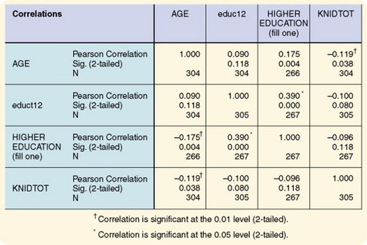
Figure 20-3 Correlational matrix using SPSS Version 9. KNIDTOT, knowledge of infant development by English-speaking Hispanic mothers.
When examining the matrix values, you must place weight only on those r values with a p value of 0.05 or smaller. Once these pairs of variables are singled out, you will note variable pairs with an r value sufficiently large to be of interest in terms of the study problem. By examining these pairs of variables, you can gain theoretical insight into the dynamics of the variables within the problem of concern in the study. Of particular interest are pairs of variables that are unexpectedly significantly related. These results can sometimes provide new insight into the research problem.
Spurious Correlations
Spurious correlations are relationships between variables that are not logical. In some cases, these significant relationships are a consequence of chance and have no meaning. When you choose a level of significance of 0.05, 1 in 20 correlations that you perform in a matrix will be significant by chance. Other pairs of variables may be correlated because of the influence of other variables. For example, you might find a positive correlation between the number of deaths on a nursing unit and the number of nurses working on the unit. Clearly, the number of deaths cannot be explained as occurring because of increases in the number of nurses. It is more likely that a third variable (units having patients with more critical conditions) explains the increased number of nurses. In most cases, the “other” variable will remain unknown. You can use reasoning to identify and exclude most of these correlations.
Spearman Rank-Order Correlation Coefficient
The Spearman rank-order correlation coefficient is an adaptation of the Pearson product-moment correlation, discussed later in this chapter. Use this test when the assumptions of Pearson’s analysis cannot be met. For example, the data may be ordinal, or the scores may be skewed. (Data might be, for example, placement on test by rank and income level by rank.) (Grove, 2007)
Calculation
The data must be ranked to conduct the analysis. Therefore, if a researcher uses scores from measurement scales to perform the analysis, the scores must be converted to ranks. As with all correlational analyses, each subject in the analysis must have a score (or value) on each of two variables (variable x and variable y). The scores on each variable are ranked separately. Rho is calculated based on difference scores between a subject’s ranking on the first and second set of scores. The formula for this calculation is as follows:

As in most statistical analyses, difference scores are difficult to use directly in equations because negative scores tend to cancel out positive scores; therefore, the scores are squared for use in the analysis. The formula is as follows:
where
Interpretation of Results
When you use an equation to analyze data that meet the assumptions of Pearson’s correlational analysis, the results are equivalent or slightly lower than Pearson’s r, discussed later in this chapter. If the data are skewed, rho has an efficiency of 91% in detecting an existing relationship. The significance of rho must be tested as with any correlation; the formula used is presented in the following equation. The t distribution is presented in Appendix C, and df = N – 2.
Kendall’s Tau
Kendall’s tau is a nonparametric measure of correlation used when both variables have been measured at the ordinal level (e.g., strength of evidence and education of researcher). You can use it with very small samples. The statistic tau reflects a ratio of the actual concordance obtained between rankings with the maximal concordance possible. This text uses Marascuilo and McSweeney’s (1977) explanation of this analysis technique.
Calculation
To calculate tau, rank the scores on each of the two variables independently. Arrange the paired scores by subject, with the lowest ranking score on variable x at the top of the list and the ranking score on variable y for the same subject in the same row. Table 20-2 presents an example of the ranking of scores for five subjects on variables x and y.
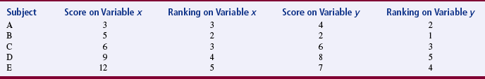
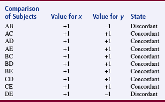
Then compare the relative ranking position between each pair of subjects on variable y, shown in the last column in the table. (It is not necessary to compare rankings on variable x because the data have been arranged in order by rank.) If the comparison is concordant, the ranking of the score below will be higher than the ranking of the score above and is assigned a value of +1. If the comparison is discordant, the ranking of the score below will be lower than the ranking of the score above and is assigned a value of –1. In Table 20-3, the comparisons are identified as concordant (+1) or discordant (–1) for the ranked scores identified in Table 20-1. In this example, the number of discordant pairs is two; the number of concordant pairs is eight. The statistic S is then calculated with the following equation:
where

At this point, tau is calculated by using the following equation:
where

Interpretation of Results
If the ranking of values of x is not related to the ranking of values of y, any particular rank ordering of y is just as likely to occur as any other. The sample tau can be used to test the hypothesis that the population tau is 0. The significance of tau can be tested by using the following equation for the Z statistic. The Z statistic was calculated for the previous example.
The Z values are approximately normally distributed, and therefore you can use the table of Z scores available in Appendix 2 (available on the Evolve website at http://evolve.elsevier.com/Burns/Practice/). The Z score for the example was 1.47, which is nonsignificant at the p ≤ 0.05 level.
Role of Correlation in Understanding Causality
In any situation involving causality, a relationship will exist between the factors involved in the causal process. Therefore, the first clue to the possibility of a causal link is the existence of a relationship. However, a relationship does not mean causality. For example, blood sugar level may be related to body temperature, however this does not mean that one causes the other. Two variables can be highly correlated but have no causal relationship whatsoever. However, as the strength of a relationship increases, the possibility of a causal link increases. The absence of a relationship precludes the possibility of a causal connection between the two variables being examined, given adequate measurement of the variables and absence of other variables that might mask the relationship. Thus, a correlational study can be the first step in determining the dynamics important to nursing practice within a particular population. Determining these dynamics can allow us to increase our ability to predict and control the situation studied. However, correlation cannot be used to demonstrate causality.
MULTIVARIATE CORRELATIONAL PROCEDURES
Multivariate correlational procedures are more complex analysis techniques that examine linear relationships among three or more variables.
Factor Analysis
Factor analysis examines interrelationships among large numbers of variables and disentangles those relationships to identify clusters of variables that are most closely linked together (factors). Several factors may be identified within a data set. Sample sizes must be large for factor analysis. Nunnally and Bernstein (1994) recommended 10 observations for each variable. Arrindell and van der Ende (1985) suggested that a more reliable determination is a sample size of 20 times the number of factors. You can also perform a power analysis to determine the sample size.
Once the factors have been identified mathematically, the researcher explains why the variables are grouped as they are. Thus, factor analysis aids in the identification of theoretical constructs. Factor analysis is also used to confirm the accuracy of a theoretically developed construct. For example, a theorist might state that the concept “hope” consists of the elements (1) anticipation of the future, (2) belief that things will work out for the best, and (3) optimism. Instruments could be developed to measure these three elements, and factor analysis could be conducted on the data to determine whether subject responses clustered into these three groupings.
Factor analysis is frequently used in the process of developing measurement instruments, particularly those related to psychological variables such as attitudes, beliefs, values, or opinions. The instrument operationalizes a theoretical construct. The method can also be used with physiological data. For example, Woods, Lentz, and Mitchell (1993) identified a large pool of symptoms commonly experienced during the perimenstruum, and daily rating of the severity of these symptoms by subjects was used to identify premenstrual symptom patterns. Testing of the validity of these patterns by factor analysis resulted in the selection of 33 symptoms for classification of women as having a low-severity symptom pattern, a premenstrual syndrome pattern, or a premenstrual magnification pattern. The analysis revealed that these patterns (factors) were consistent across menstrual cycle phases and had internal consistency reliability estimates above 0.70 (Woods, Mitchell, & Lentz, 1995). This work has now been recognized in medicine as well as nursing in defining menstrual difficulties clinically as well as in research. Factor analysis can be used as a data reduction strategy in studies examining large numbers of variables. It can also be used to attempt to sort out meaning from large numbers of items on survey instruments.
The two types of factor analysis are exploratory and confirmatory. Exploratory factor analysis is similar to stepwise regression, in which the variance of the first factor is partialed out before analysis on the second factor begins. It is performed when the researcher has few prior expectations about the factor structure. Confirmatory factor analysis is more closely related to ordinary least-squares regression analysis or path analysis. It is based on theory and tests a hypothesis about the existing factor structure. In confirmatory factor analysis, the researcher determines the statistical significance of the analysis outcomes and estimates the parameters of the population. Confirmatory factor analysis is usually conducted after the correlation matrix has been examined or after initial development of the factor structure through exploratory factor analysis.
Exploratory Factor Analysis
The first step in exploratory factor analysis is the development of a correlation matrix of the scores for all variables to be included in the factor analysis. The computer program conducting the analysis usually develops this matrix automatically. Although multiple procedures can be used for the actual factor analysis, the procedure described here is the one most commonly reported in the nursing literature.
The second step is a principal components analysis, which provides the preliminary information that the researcher needs to make decisions before the final factoring. The computer printout of the principal components analysis will give (1) the eigenvalues, (2) the amount of variance explained by each factor, and (3) the weight for each variable on each factor. Weights (loadings) express the extent to which the variable is correlated with the factor. Weightings on the variables from a principal components factor analysis are essentially uninterpretable and are generally disregarded (Nunnally & Bernstein, 1994).
Eigenvalues are the sum of the squared weights for each factor. The researcher examines the eigenvalues to decide how many factors will be included in the factor analysis. To decide the number of factors to include, the researcher determines the minimal amount of variance that must be explained by the factor to add significant meaning. This decision is not straightforward, however, and some have criticized the analysis for being subjective. Several strategies have been proposed for determining the number of factors to be included in a construct. One approach is to select factors that have an eigenvalue of 1.00 or above. Another strategy used is the screen test. Scree is a geological term that refers to the debris that collects at the bottom of a rocky slope. This test, which is considered by some to be the most reliable, requires that the eigenvalues be graphed (Figure 20-4).
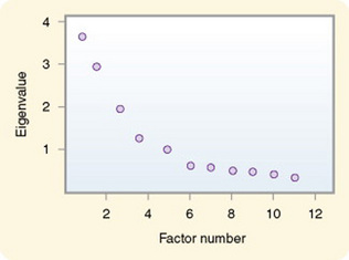
This graph shows a change in the angle of the slope. A steep drop in value from one factor to the next indicates a large difference score between the two factors and an increase in the amount of variance explained. When the slope begins to become flat, which is an indication of small difference scores between factors, little additional information will be obtained by including more factors. In Figure 20-4, the slope begins to flatten at factor 6; therefore, six factors would be extracted to explain the construct.
The third step in exploratory factor analysis is factor rotation. Factor rotation simplifies the factor structure, and the procedure most commonly used is referred to as varimax rotation. In varimax rotation, the factors are rotated for the best fit (best factor solution), and the factors are uncorrelated. An oblique rotation results in correlated factors.
The process of factor analysis is actually a series of multiple regression analyses (Kim & Mueller, 1978a, 1978b). The equation for a factor could be expressed as
where
In exploratory factor analysis, regression analysis is performed for the first factor. The variance of each variable explained by the first factor is then partialed out. Next, a second regression analysis is performed for the second factor on the residual variance. The variance from that analysis is then partialed out, and a regression is performed for the third factor. This process is continued until all the factors have been developed. The computer printout will include a rotated factor matrix that contains information similar to that in Table 20-4.
TABLE 20-4
Factor Loading and Variance for Two Factors
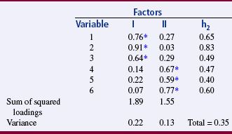
*Indicates the variables to be included in each factor.
Factor Loadings: A factor loading is actually the regression coefficient of the variable on the factor. In Table 20-4, the factor loading indicates the extent to which a single variable is related to the cluster of variables. In variable 1, the factor loading is 0.76 for factor I and 0.27 for factor II. Squaring the factor loadings ([0.76]2 = 0.578, and [0.27]2 = 0.073) gives the amount of variance in variable 1, which explains factors I and II.
Communality: Communality (h2) is the squared multiple regression coefficient for each variable and closely relates to the R2 coefficient in regression. Thus, the communality coefficient describes the amount of variance in a single variable that is explained across all the factors in the analysis. To obtain the communality for a variable, sum the squared factor loadings on the variable for each factor. In Table 20-4, the communality coefficient for variable 1 is (0.76)2 + (0.27)2 = 0.65.
Identifying the Relevant Variables in a Factor: Only variables with factor loadings that indicate that a meaningful portion of the variable’s variance is explained within the factor are included as elements of the factor. A cutoff point is selected to identify these variables, with the minimal acceptable cutoff point being 0.30. In Table 20-4, the factor loadings with asterisks indicate the variables that will be included in each factor. In this example, which uses a 0.50 cutoff, variables 1, 2, and 3 would be included in factor I, and variables 4, 5, and 6 would be included in factor II. Ideally, a variable will load (have a factor loading above the selected cutoff point) on only one factor. If the variable does have high loadings on two factors, the lowest loading is referred to as a secondary loading. When many secondary loadings occur, it is not considered a clean factoring, and the researcher reexamines the variables included in the analysis. Sometimes, researchers attempt to set the cutoff point high enough to avoid secondary loadings of a variable.
“Naming” the Factor: At this point, the mathematics of the procedure takes a back seat, and the researcher’s theoretical reasoning takes over. The researcher examines the variables that have clustered together in a factor and explains that clustering. Variables with high loadings on the factor must be included, even if they do not fit the researcher’s preconceived theoretical notions. The purpose is to identify the broad construct of meaning that has caused these particular variables to be so strongly intercorrelated. Naming this construct is an important part of the procedure because naming of the factor provides theoretical meaning.
Factor Scores: After the initial factor analysis, additional studies are conducted to examine changes in the phenomenon in various situations and to determine the relationships of the factors with other concepts. Factor scores are used during data analysis in these additional studies. To obtain factor scores, the variables included in the factor are identified, and the scores on these variables are summed for each subject. Thus, each subject will have a score for each factor in the instrument. Because some variables explain a larger portion of the variance of the factor than others do, additional meaning can be added by multiplying the variable score by the weight (factor loading) of that variable in the factor. In the example in Table 20-4, variable 1 had a factor loading of 0.76 on factor I. If the subject score on variable 1 were 7, the score would be weighted by multiplying the variable score by the factor loading as follows:

A computer can generate these weighted scores. If studies are to be compared, standardized (Z) scores (for variable scores) and beta weights (for factor loadings) are used. Once analysis is complete, factor scores can be used as independent variables in multiple regression equations.
Ramirez, Tart, and Malecha (2006) used factor analysis to identify treatment competencies of nurse practitioners providing care in emergency rooms. The factor analysis is reported as follows:
SUMMARY
• Correlational analyses identify relationships between or among variables.
• The purpose of the analysis is also to clarify relationships among theoretical concepts or help to identify potentially causal relationships, which can then be tested by inferential analysis.
• All data for the analysis should have been obtained from a single population from which values are available on all variables to be examined.
• Data measured at the interval or ratio level provide the best information on the nature of the relationship.
• Correlational analysis provides two pieces of information about the data: the nature of a linear relationship (positive or negative) between the two variables and the magnitude (or strength) of the linear relationship.
• The Spearman rho, a nonparametric test, is used when the assumptions of Pearson’s analysis cannot be met.
• Kendall’s tau is a nonparametric measure of correlation used when both variables have been measured at the ordinal level.
• Pearson’s correlation is used when both variables have been measured at the interval or ratio level.
• A correlational matrix is obtained by performing bivariate correlational analysis on every pair of variables in the data set.
• The first clue to the possibility of a causal link is the existence of a relationship, but a relationship does not necessarily mean causality.
• Multivariate correlational procedures are more complex analysis techniques that examine linear relationships among three or more variables.
• Factor analysis examines interrelationships among large numbers of variables and disentangles those relationships to identify clusters of variables that are most closely linked (factors).
REFERENCES
Arrindell, W.A., van der Ende, J. An empirical test of the utility of the observations-to-variables ratio in factor and components analysis. Applied Psychological Measurement. 1985;9(2):165–178.
Grove, S.K. Statistics for health care research: A practical workbook. Philadelphia: Saunders, 2007.
Kim, J., Mueller, C.W. Factor analysis: Statistical methods and practical issues. Beverly Hills, CA: Sage, 1978.
Kim, J., Mueller, C.W. Introduction to factor analysis: What it is and how to do it. Beverly Hills, CA: Sage, 1978.
Marascuilo, L.A., McSweeney, M. Nonparametric and distribution-free methods for the social sciences. Monterey, CA: Brooks/Cole, 1977.
Nunnally, J.C., Bernstein, I. Psychometric theory, (3rd ed.). New York: McGraw-Hill, 1994.
Ramirez, E.G., Tart, K., Malecha, A. Developing nurse practitioner treatment competencies in emergency care settings. Advanced Emergency Nursing Journal. 2006;28(4):346–359.
Woods, N.F., Lentz, M.J., Mitchell, E.S. Prevalence of perimenstrual symptoms. Unpublished report to National Center for Nursing Research, 1993.
Woods, N.F., Mitchell, E.S., Lentz, M.J. Social pathways to premenstrual symptoms. Research in Nursing & Health. 1995;18(3):225–237.