Using Statistics to Examine Causality
Causality is a way of knowing that one thing causes another. Statistical procedures that examine causality are critical to the development of nursing science because of their importance in examining the effects of interventions. The statistical procedures in this chapter examine causality by testing for significant differences between or among groups. Statistical procedures are available for nominal, ordinal, and interval data. The procedures vary considerably in their power to detect differences and in their complexity. They are categorized as contingency tables, chi-squares, t-tests, and analysis of variance (ANOVA) procedures.
CONTINGENCY TABLES
Contingency tables, or cross-tabulation, allow the researcher to visually compare summary data output related to two variables within the sample. Contingency tables are a useful preliminary strategy for examining large amounts of data. In most cases, the data are in the form of frequencies or percentages. With this strategy, one can compare two or more categories of one variable with two or more categories of a second variable. The simplest version is referred to as a 2 × 2 table (two categories of two variables). Table 22-1 shows an example of a 2 × 2 contingency table from Knafl’s (1985) study of how families manage a pediatric hospitalization.
TABLE 22-1
Relationship between Parents’ Reports of Impact on Family Life and Outside Help
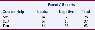
*Includes cases from “Alone” category.
†Combines cases from “Some Help” and “Delegation” categories.
Modified from Knafl, K. A. (1985). How families manage a pediatric hospitalization. Western Journal of Nursing Research, 7(2), 163.
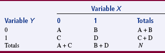
The data are generally referenced in rows and columns. The intersection between the row and column in which a specific numerical value is inserted is referred to as a cell. The upper left cell would be row 1, column 1. In Table 22-1, the cell of row 1, column 1 has the value of 18, the cell of row 1, column 2 has the value of 7, and so on. The output from each row and each column is summed, and the sum is placed at the end of the row or column. In the example, the sum of row 1 is 25, the sum of row 2 is 37, the sum of column 1 is 34, and the sum of column 2 is 28. The percentage of the sample represented by that sum can also be placed at the end of the row or column. The row sums and the column sums total to the same value, which is 62 in the example.
Although researchers commonly use contingency tables to examine nominal or ordinal data, they can be used with grouped frequencies of interval data. However, information about the data will be lost when contingency tables are used to examine interval data. Loss of data usually causes loss of statistical power—that is, the probability of failing to reject a false null hypothesis is greater than if an appropriate parametric procedure could be used. Therefore, it is not generally the technique of choice. A contingency table is sometimes useful when an interval-level measure is being compared with a nominal- or ordinal-level measure.
In some cases, the contingency table is presented and no further analysis is conducted. The table is presented as a form of summary statistics. However, in many cases, a statistical analysis of the relationships or differences between the cell values is performed. The most familiar analysis of cross-tabulated data is use of the chi-square (χ2) statistic. Chi-square is designed to test for significant differences between cells. Some statisticians prefer to examine chi-square from a probability framework and use it to detect possible relationships (Goodman & Kruskal, 1954, 1959, 1963, 1972).
Computer programs are also available to analyze data from cross-tabulation tables (contingency tables). These programs can generate output from chi-square and many correlational techniques and indicate the level of significance for each technique. As the researcher, you should know which statistics are appropriate for your data and how to interpret the outcomes from these multiple analyses. The information presented on each of these tests will guide you in selecting a test and interpreting the findings.
Chi-Square Test of Independence
The chi-square test of independence tests whether the two variables being examined are independent or related. Chi-square is designed to test for differences in frequencies of observed data and compare them with the frequencies that could be expected to occur if the data categories were actually independent of each other. If differences are indicated, the analysis will not identify where these differences exist within the data.
Assumptions
One assumption of the test is that only one datum entry is made for each subject in the sample. Therefore, if repeated measures from the same subject are being used for analysis, such as pretests and posttests, chi-square is not an appropriate test. Another assumption is that for each variable, the categories are mutually exclusive and exhaustive. No cells may have an expected frequency of zero. However, in the actual data, the observed cell frequency may be zero. Until recently, each cell was expected to have a frequency of at least five, but this requirement has been mathematically demonstrated not to be necessary. However, no more than 20% of the cells should have fewer than five (Conover, 1971). The test is distribution-free, or nonparametric, which means that no assumption has been made of a normal distribution of values in the population from which the sample was taken.
Calculation
The formula is relatively easy to calculate manually and can be used with small samples, which makes it a popular approach to data analysis. The first step in the calculation of chi-square is to categorize the data, record the observed values in a contingency table, and sum the rows and columns. Next, the expected frequencies are calculated for each cell. The expected frequencies are those frequencies that would occur if there were no group differences; these frequencies are calculated from the row and column sums by using the following formula:
where
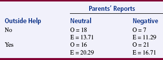
Thus, to obtain the expected frequency for a particular cell, you would multiply the row total by the column total and divide by the sample size. When the expected frequencies have been calculated for all the cells, the sum should be equivalent to the total sample size. Calculations of the expected frequencies for the four cells in Table 22-1 follow; they total 62 (sample size):
By using this same example, a contingency table could be constructed of the observed and expected frequencies (Table 22-2). The following formula is then used to calculate the chi-square statistic:
where
Note that the formula includes difference scores between the observed frequency for each cell and the expected frequency for that cell. These difference scores are squared, divided by the expected frequency, and summed for each cell. The chi-square value was calculated by using the observed and expected frequencies in Table 22-2.
With any chi-square analysis, the degrees of freedom (df) must be calculated to determine the significance of the value of the statistic. The following formula is used for this calculation:
where
In the example presented previously, the chi-square value was 4.98, and df was 1, which was calculated as follows:
Interpretation of Results
The chi-square statistic is compared with the chi-square values in the table in Appendix Chttp://evolve.elsevier.com/Burns/Practice/. The table includes the critical values of chi-square for specific degrees of freedom at selected levels of significance (usually 0.05 or 0.01). A critical value is the value of the statistic that must be obtained to indicate that a difference exists in the two populations represented by the groups under study. If the value of the statistic is equal to or greater than the value identified in the chi-square table, the difference between the two variables is significant. If the statistic remains significant at more extreme probability levels, you will report the largest p value at which significance is achieved. The analysis indicates that there are group differences in the categories of the variable and that those differences are related to changes in the other variable. Although a significant chi-square value indicates difference, the analysis does not reveal the magnitude of the difference. If the statistic is not significant, we cannot conclude that there is a difference in the distribution of the two variables, and they are considered independent (Salkind, 2007).
How one interprets the results depends on the design of the study. If the design is experimental, causality can be considered and the results can be inferred to the associated population. If the design is descriptive, differences identified are associated only with the sample under study. In either case, the differences found are related to differences among all the categories of the first variable and all the categories of the second variable. The specific differences among variables and categories of variables cannot be identified with this analysis. Often, in reported research, the researcher will visually examine the data and discuss differences in the categories of data as though they had been demonstrated to be statistically significantly different. The reader must view these reports with caution. Partitioning, the contingency coefficient C, the phi coefficient, or Cramer’s V can be used to examine the data statistically to determine in exactly which categories the differences lie. The last three strategies can also shed some light on the magnitude of the relationship between the variables. These strategies are discussed later in this chapter.
In reporting the results, contingency tables are generally presented only for significant chi-square analyses. The value of the statistic is given, including the df and p values. Data in the contingency table are sufficient to allow other researchers to repeat the chi-square analyses and thus check the accuracy of the analyses.
The chi-square test of independence can be used with two or more groups. In this case, group membership is used as the independent variable. The chi-square statistic is calculated with the same formula as above. If more than two categories of the dependentvariable are present, the analysis tests differences in both central tendency and dispersion.
Partitioning of Chi-Square
Partitioning involves breaking up the contingency table into several 2 × 2 tables and conducting chi-square analyses on each table separately. Partitioning can be performed on any contingency table greater than 2 × 2 with more than one degree of freedom. The number of partitions that can be conducted is equivalent to the degrees of freedom. The sum of the chi-square values obtained by partitioning is equal to the original chi-square value. Certain rules must be followed during partitioning to prevent inflating the value of chi-square. The initial partition can include any four cells as long as two values from each variable are used. The next 2 × 2 must compress the first four cells into two cells and include two new cells. This process can continue until no new cells are available. By using this process, it is possible to determine which cells have contributed to the significant differences found.
Phi
The phi coefficient (ϕ) describes relationships in dichotomous, nominal data. It is also used with the chi-square test to determine the location of a difference or differences among cells. Phi is used only with 2 × 2 tables (Table 22-3).
Calculation
If chi-square has been calculated, the following formula can be used to calculate phi. The data presented in Table 22-1 were used to calculate this phi coefficient. The chi-square analysis indicated a significant difference, and the phi coefficient indicated the magnitude of effect:
where N is the total frequency of all cells.
Alternatively, phi can be calculated directly from the 2 × 2 table by using the following formula (Salkind, 2007). Again, the data from Table 22-1 are used to calculate the phi coefficient:
Interpretation of Results
The phi coefficient is similar to Pearson’s product moment correlation coefficient (r), except that two dichotomous variables are involved. Phi values range from −1 to +1, with the magnitude of the relationship decreasing as the coefficient nears zero. The results show the strength of the relationship between the two variables.
Cramer’s V
Cramer’s V is a modification of phi used for contingency tables larger than 2 × 2. It is designed for use with nominal data. The value of the statistic ranges from 0 to 1.
Calculation
The formula can be calculated from the chi-square statistic, and the data presented in Table 22-1 were used to calculate Cramer’s V:
where
Contingency Coefficient
The contingency coefficient (C) is used with two nominal variables and is the most commonly used of the three chi-square–based measures of association.
Calculation
The contingency coefficient can be calculated with the following formula, which uses the data presented in Table 22-1:

The relationship demonstrated by C cannot be interpreted on the same scale as Pearson’s r, phi, or Cramer’s V because it does not reach an upper limit of 1. The formula does not consider the number of cells, and the upper limit varies with the size of the contingency table. With a 2 × 2 table, the upper limit is 0.71; with a 3 × 3 table, the upper limit is .82; and with a 4 × 4 table, the upper limit is 0.87. Contingency coefficients from separate analyses can be compared only if the table sizes are the same.
Lambda
Lambda measures the degree of association (or relationship) between two nominal-level variables. The value of lambda can range from 0 to 1. Two approaches to analysis are possible: asymmetrical and symmetrical. The asymmetrical approach indicates the capacity to predict the value of the dependent variable given the value of the independent variable. Thus, when you use the asymmetrical lambda, it is necessary to specify a dependent and an independent variable. Symmetrical lambda measures the degree of overlap (or association) between the two variables and makes no assumptions regarding which variable is dependent and which is independent (Waltz & Bausell, 1981).
t-TESTS
t-Test for Independent Samples
One of the most common parametric analyses used to test for significant differences between statistical measures of two samples is the t-test. The t-test uses the standard deviation of the sample to estimate the standard error of the sampling distribution. The ease in calculating line formula is attractive to researchers who wish to conduct their analyses by hand. This test is particularly useful when only small samples are available for analysis. The t-test being discussed here is for independent samples.
The t-test is frequently misused by researchers who use multiple t-tests to examine differences in various aspects of data collected in a study. This practice escalates significance and greatly increases the risk of a type I error. The t-test can be used only one time during analysis to examine data from the two samples in a study. You can use the Bonferroni procedure, which controls for the escalation of significance, if you must perform various t-tests on different aspects of the same data. You can easily complete a Bonferroni adjustment by hand; simply divide the overall significance level by the number of tests, and use the resulting number as the significance level for each test. ANOVA is always a viable alternative to the pooled t-test and is preferred by many researchers who have become wary of the t-test because of its frequent misuse. Mathematically, the two approaches are the same when only two samples are being examined.
Use of the t-test involves the following assumptions:
1. Sample means from the population are normally distributed.
2. The dependent variable is measured at the interval level.
The t-test is robust to moderate violation of its assumptions. Robustness means that the results of analysis can still be relied on to be accurate when one of the assumptions has been violated. The t-test is not robust with respect to the between-samples or within-samples independence assumptions, nor is it robust with respect to an extreme violation of the normality assumption unless the sample sizes are extremely large. Sample groups do not have to be equal for this analysis—the concern is, instead, for equal variance. A variety of t-tests have been developed for various types of samples. Independent samples means that the two sets of data were not taken from the same subjects and that the scores in the two groups are not related.
Calculation
The t statistic is relatively easy to calculate. The numerator is the difference scores of the means of the two samples. The test uses the pooled standard deviation of the two samples as the denominator, which gives the formula a rather forbidding appearance:


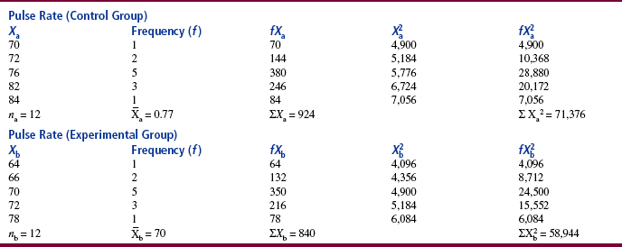
In the following example, the t-test was used to examine the difference between a control group and an experimental group. The independent variable administered to the experimental group was a form of relaxation therapy. The dependent variable was pulse rate. Pulse rates for the experimental and control groups are presented in Table 22-4, along with calculations for the t-test.


Interpretation of Results
To determine the significance of the t statistic, the researcher must calculate the degrees of freedom. The value of the t statistic is then found in the table for the sampling distribution. If the sample size is 30 or fewer, you can use the t distribution; a table of this distribution can be found in Appendix A. For larger sample sizes, you can use the normal distribution; a table of this distribution is presented in Appendix 2 (available on the Evolve website at http://evolve.elsevier.com/Burns/Practice/). The level of significance and the degrees of freedom are used to identify the critical value of t. This value is then used to obtain the most exact p value possible. The p value is then compared with the significance level. In the example presented in Table 22-4, the calculated t = 4.169 and df = 22. This t value was significant at the 0.001 level.
Andrus and Clark (2007) conducted a study to determine the effectiveness of having a pharmacist and nurse practitioner run a rural health center. They used a t-test for the following purpose (Table 22-5).
TABLE 22-5
Comparison of Empowerment Scores between Collaborative Governance (Cg) Members and Nonmembers at 1 Year
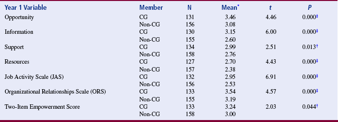
*Scale: 1 = low, 5 = high.
†Significant p ≤ 0.05.
‡Significant p ≤ 0.01.
From Erickson, J. I., Hamilton, G. A., Jones, D. E., & Ditomassi, M. (2003). The value of collaborative governance/staff empowerment. Journal of Nursing Administration, 33(2), 96–104. Full text available in Nursing Collection 2.
t-Tests for Related Samples
When samples are related, the formula used to calculate the t statistic is different from the formula just described. Samples may be related because matching has been performed as part of the design or because the scores used in the analysis were obtained from the same subjects under different conditions (e.g., pretest and posttest). This test requires that differences between the paired scores be independent and normally or approximately normally distributed.

One-Way Analysis of Variance
Although one-way ANOVA is a bivariate analysis, it is more flexible than other analyses in that it can examine data from two or more groups. To accomplish this analysis, the researcher uses group membership as one of the two variables under examination and a dependent variable as the second variable.
ANOVA compares the variance within each group with the variance between groups. The outcome of the analysis is a numerical value for the F statistic, which will be used to determine whether the groups are significantly different. The variance within each group is a result of individual scores in the group varying from the group mean and is referred to as the within-group variance. This variance is calculated in the same way as that described in Chapter 19. ANOVA assumes the amount of variation about the mean in each group to be equal. The group means also vary around the grand mean (the mean of the total sample), which is referred to as the between-groups variance. One could assume that if all the samples were drawn from the same population, there would be little difference in these two sources of variance. The variance from within and between the groups explains the total variance in the data. When these two types of variance are combined, they are referred to as the total variance.
Interpretation of Results
The test for ANOVA is always one-tailed. The critical region is in the upper tail of the test. The F distribution for determining the level of significance of the F statistic can be found in Appendix B. If you are examining only two groups, the location of a significant difference is clear. However, if you are studying more than two groups, it is not possible to determine from the ANOVA exactly where the significant differences lie. One cannot assume that all the groups examined are significantly different. Therefore, post hoc analyses are conducted to determine the location of the differences among groups.
Post Hoc Analyses: One might wonder why a researcher would conduct a test that failed to provide the answer he or she is seeking—namely, where the significant differences were in a data set. It would seem more logical to perform t-tests or ANOVAs on the groups in the data set in pairs, thus clearly determining whether a significant difference exists between those two groups. However, when these tests are performed with three groups in the data set, the risk of a type I error increases from 5% to 14%. As the number of groups increases (and with the increase in groups, an increase in the number of comparisons necessary), the risk of a type I error increases strikingly. This type I error, which increases because of escalation of the level of significance, does not occur when one ANOVA is performed that includes all of the groups.
Post hoc tests have been developed specifically to determine the location of differences after ANOVA is performed on analysis of data from more than two groups. These tests were developed to reduce the incidence of a type I error. Frequently used post hoc tests are the Bonferroni procedure, the Newman-Keuls test, the Tukey Honestly Significant Difference (HSD) test, the Scheffe test, and the Dunnett test. When these tests are calculated, the alpha level is reduced in proportion to the number of additional tests required to locate statistically significant differences. As the alpha level decreases, reaching the level of significance becomes increasingly more difficult.
Robbins et al. (2006) conducted an ANOVA in a study examining the effectiveness of a program designed by a pediatric nurse practitioner to reverse the sedentary lifestyle of adolescent girls. The results were reported as follows.
SUMMARY
• Causality is a way of knowing that one thing causes another.
• Contingency tables (or cross-tabulation) allow the researcher to visually compare summary data output related to two variables within the sample.
• The t-test is one of the most commonly used parametric analyses to test for significant differences between statistical measures of two samples.
• ANOVA procedures test for differences between means.
• ANOVA can be used to examine data from more than two groups and compares the variance within each group with the variance between groups.
Andrus, M.R., Clark, D.B. Provision of pharmacotherapy services in a rural nurse practitioner clinic. American Journal of Health-System Pharmacy. 2007;64(3):294–297.
Conover, W.J. Practical nonparametric statistics. New York: Wiley, 1971.
Erickson, J.I., Hamilton, G.A., Jones, D.E., Ditomassi, M. The value of collaborative governance/staff empowerment. Journal of Nursing Administration. 2003;33(2):96–104.
Goodman, L.A., Kruskal, W.H. Measures of association for cross classifications. Journal of the American Statistical Association. 1954;49:732–764.
Goodman, L.A., Kruskal, W.H. Measures of association for cross classifications, II: Further discussion and references. Journal of the American Statistical Association. 1959;54(285):123–163.
Goodman, L.A., Kruskal, W.H. Measures of association for cross classifications, III: Approximate sampling theory. Journal of the American Statistical Association. 1963;58(302):310–364.
Goodman, L.A., Kruskal, W.H. Measures of association for cross classifications, IV: Simplification of asymptotic variances. Journal of the American Statistical Association. 1972;67(338):415–421.
Knafl, K.A. How families manage a pediatric hospitalization. Western Journal of Nursing Research. 1985;7(2):151–176.
Robbins, L.B., Gretebeck, K.A., Kazanis, A.S., Pender, N. Girls on the move program to increase physical activity participation. Nursing Research. 2006;55(3):206–216.
Salkind, N.J. Statistics for people who (think they) hate statistics. CA: Sage: Thousand Oaks, 2007.
Volicer, B.J. Multivariate statistics for nursing research. New York: Grune & Stratton, 1984.
Waltz, C., Bausell, R.B. Nursing research: Design, statistics and computer analysis. Philadelphia: F.A. Davis, 1981.