Digital Radiographic Artifacts
At the completion of this chapter, the student should be able to do the following:
1 Discuss the three types of digital radiographic imaging artifacts and how to avoid them.
2 Identify the difference between for-processing images and for-presentation images.
3 Describe the basis for data compression and the difference between lossless and lossy compression.
4 Analyze the use of an image histogram in digital radiographic image artifacts.
5 Explain how digital radiographic image artifacts occur because of improper collimation, partition, or alignment.
AS WE learned in Chapter 19, an artifact is any false visual feature on a medical image that simulates tissue or obscures tissue. Artifacts interfere with diagnosis and must be avoided. Similar to accidents, artifacts are, by definition, avoidable.
Artifacts can be controlled when the cause of the artifact is understood. In screen-film radiography, three classifications of artifacts occur—processing, exposure, and handling or storage. Likewise, in digital radiography (DR), three classifications of artifacts can be described—image receptor, software, and object.
When digital radiographic images are printed, processing artifacts may have to be considered, as they are with screen-film radiographic images. Such considerations are not repeated here.
The three digital imaging artifact classes are shown in Figure 21-1 along with the subsets of each.
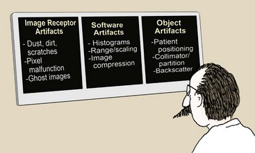
Image Receptor Artifacts
As can occur with screen-film image receptors, digital image receptors can suffer from rough handling, scratches, and dust (Figure 21-2). Artifacts produced by dust can be corrected easily with proper cleaning unless the dust is internal to the optics of a computed radiography (CR) imaging system. Figure 21-3 shows a CR image taken with an imaging plate (IP) contaminated with residual glue that could not be removed. Dust on any section of the CR optical path—mirrors and lenses—cannot be corrected by the radiologic technologist and will require professional service.
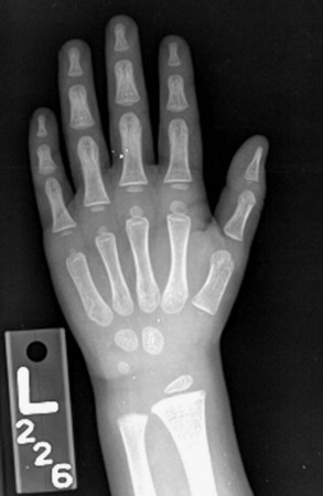
FIGURE 21-2 Debris on image receptor in digital radiography can be confused with foreign bodies. (Courtesy Charles Willis, M.D. Anderson Cancer Center.)
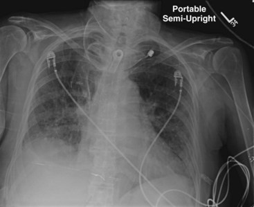
FIGURE 21-3 Residual glue on a computed radiography imaging plate resulted in this artifact, causing the plate to be removed from service. (Courtesy David Clayton, M.D. Anderson Cancer Center.)
Scratches or a substantial malfunction of pixels likely will require replacement of the image receptor.
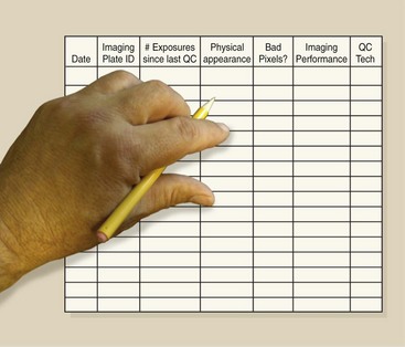
Digital radiography including CR IPs should last for thousands of exposures. There is no such thing as “radiation fatigue” on these IPs. Routine quality control (QC) should include regular documentation of imaging frequency, imaging performance, and the physical condition of each IP, to reduce artifact appearance and help prevent failure. Figure 21-4 is an example of a QC form for such regular documentation.
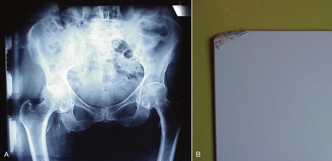
The appearance of ghost images (Figure 21-5) occurs because of incomplete erasure of a previous image on a CR IP. Usually, such artifacts can be corrected by additional signal erasure techniques. If a CR IP has not been used for 24 hours, it should be erased again before use. When a completely erased IP is processed, the resultant image should be uniform and artifact free.
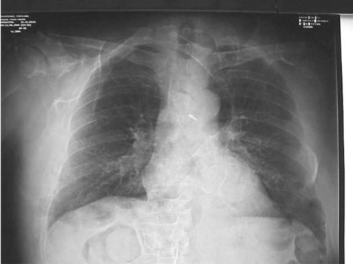
FIGURE 21-5 Look closely and you can see the pelvis at the top of this image and the bowel pattern at the bottom. This resulted because the imaging plate was not fully erased before the chest examination was performed. (Courtesy Barbara Smith Pruner, Portland Community College.)
Rough handling or faulty construction of a digital IP can result in artifacts. Figure 21-6 shows the result on the image from a damaged CR IP.
Software Artifacts
Digital radiographic images are obtained as raw data sets. As such, these images are ready “for processing.” For-processing images are manipulated into “for-presentation” images that the radiologic technologist can use for QC and for interpretation by the radiologist.
Preprocessing
Before an image is prepared “for processing,” several manipulations of the output of an image receptor may be necessary to correct for potential artifacts. Such artifacts can occur because of dead pixels or dead rows or columns of pixels (Figure 21-7).
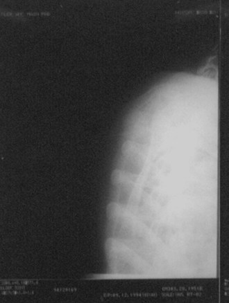
FIGURE 21-7 Failure of electronic preprocessing can cause uninterpretable images in digital radiography. (Courtesy Charles Willis, M.D. Anderson Cancer Center.)
A single pixel or a single row or column normally will not interfere with diagnosis. However, many of these defects must be corrected. Correction algorithms specific to each type of digital image receptor use interpolation techniques to assign digital values to each dead pixel, row, or column. Interpolation is the mathematical process of assigning a value to a dead pixel based on the recorded values of adjacent pixels.
Irradiation of a digital radiographic image receptor by the raw x-ray beam may show variations over the image, producing an irregular pattern that could interfere with diagnosis (Figure 21-8, A). With this irregular pattern, a preprocessing manipulation known as flatfielding is performed, resulting in a uniform response to a uniform x-ray beam (Figure 21-8, B).
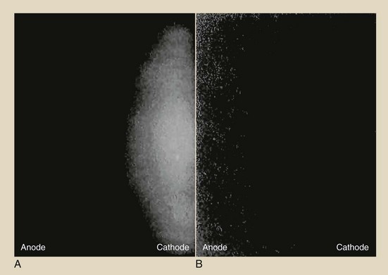
FIGURE 21-8 A, An image receptor exposed to a raw x-ray beam may show a heel-effect response. B, Flatfielding preprocessing can make the response uniform. (Courtesy Charles Willis, M.D. Anderson Cancer Center.)
 Flatfielding is a software correction that is performed to equalize the response of each pixel to a uniform x-ray beam.
Computed radiography cassettes are highly sensitive to background radiation and scatter. If a CR cassette has not been used for several days, it should be inserted into the reader for re-erasure (Figure 21-9). The practice of leaving cassettes in a supposedly “radiation-safe” area in an x-ray room during an examination must be discouraged.
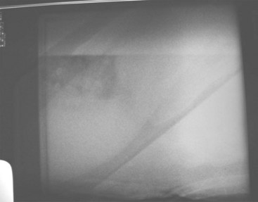
Image Compression
Digital radiographic imaging becomes evermore robust in terms of the digital data files generated. This would not represent a problem if it were not for increasing application of teleradiology, which requires the electronic transmission of images. Table 21-1 presents the relative file sizes per image for various digital imaging modalities.
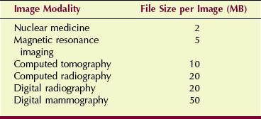
At up to 50 MB per image on a 24- × 30-cm IP (216 and 50-µm pixel size), a four-view digital mammography study can generate 200 MB. Transmitting and archiving this amount of data is technically difficult; therefore, compression techniques are used.
Data compression takes advantage of redundancy of data, as occurs with exposure to the raw x-ray beam when all values are the same. Such compression techniques are described as lossless or lossy.
An image file that is compressed in a lossless mode is one that can be reconstructed to be exactly the same as the original image. Lossless compression reduces the data file to 10% (10 : 1) to 50% (2 : 1) of the original file. However, this is not satisfactory for large image files because transmission time and data manipulation time can still be unacceptable.
Lossy compression, which can provide compression factors of up to 100 : 1 or greater, can be used on images in which exact measurement or fine detail is not required, such as video recordings that are to be replayed on a standard domestic television.
Lossless compression up to 3 : 1 generally is considered acceptable and helpful in digital radiographic image management.
Lossy compression is that which is something greater than an order of magnitude compression less than 10 : 1. Such a level of compression supports teleradiology but not computer-aided detection (CAD) or image archiving. CAD systems require uncompressed for-processing images. Compressed images may cause the CAD system to miss lesions because of the compression artifact, which actually represents a lack of data. Lossy compression is not acceptable for archiving mammography images for this reason.
Object Artifacts
Object artifacts can arise from the technologist’s errors in patient positioning, x-ray beam collimation, and histogram selection. Backscatter radiation also can be troublesome because of the sensitivity of the digital radiographic image receptor.
If a lot of scattering material is present behind the image receptor, backscatter radiation can cause a phantom image. If this type of artifact is discovered, the back side of the image receptor should be shielded to reduce backscatter x-rays.
Image Histogram
Digital radiographic image histograms are very important for digital image production. However, they can be the source of bothersome digital radiographic image artifacts if they are not properly understood and manipulated.
All digital radiographic imaging systems have the ability to evaluate the original image data through histogram analysis. A histogram is a plot of the frequency of appearance of a given object characteristic.
A sample histogram is shown in Figure 21-10, where the heights of 500 emperor penguins and 500 little blue penguins are plotted. The average height of emperor penguins is approximately 110 cm (range, 60–160 cm). The same value for the little blue penguins is approximately 30 cm (range, 15–80 cm).
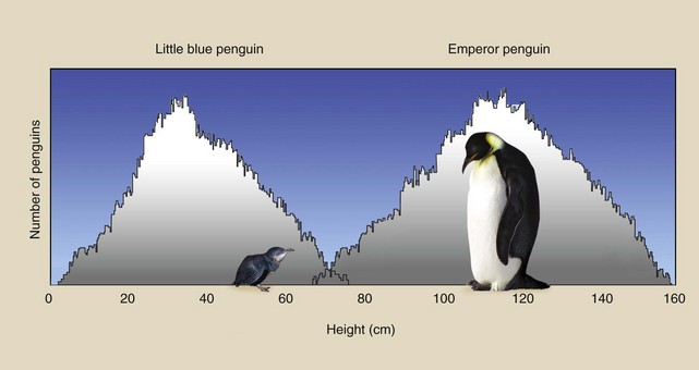
FIGURE 21-10 This histogram is a plot of the number of penguins as a function of the height of each penguin.
A histogram is a discrete plot of values rather than a continuous plot. The histogram in Figure 21-10 is a plot of the number of penguins (frequency) that have a given height as a function of that height (value interval). Because there are two penguin populations, two peaks are evident on this histogram.
Consider the simulated chest radiograph of Figure 21-11, and note where each identified part of the image would appear on a screen-film response curve—the characteristic curve. The collimated portion is white with no contrast, and the fully exposed portion is black, also with no contrast. Those two portions of every radiograph set limits on the useful portion of the image.
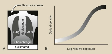
FIGURE 21-11 A, Simulated chest radiograph shows areas of lung and tissue that are unexposed (collimated) or fully exposed (raw x-ray beam). B, The point where each would fall on a characteristic curve.
When the chest radiograph is digital, each region of the image (Figure 21-12, A) can be represented by the frequency distribution of the digital values of each pixel, as shown in Figure 21-12, B. The location of those image regions on the digital image receptor response curve is shown in Figure 21-12, C. The relative shape of this histogram is characteristic of all posteroanterior (PA) chest digital radiographs.
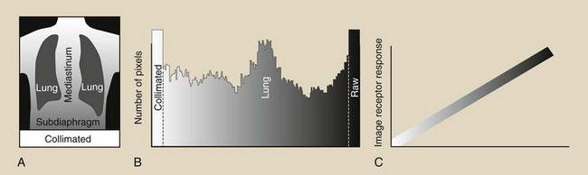
FIGURE 21-12 A, Region of a simulated digital chest radiograph. B, The corresponding image histogram. C, The placement of each region in A on the response curve of the digital image receptor.
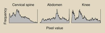
Even more important is the fact that the shape of an image histogram is characteristic of each anatomical projection. Figure 21-13 shows the characteristic shapes of image histograms of additional radiographic projections.
Most digital radiographic imaging systems have the ability to store and analyze characteristic image histograms for each radiographic projection. By storing 50 PA chest image histograms and averaging the value of each frequency interval, a representative histogram is produced for each image receptor. The histogram can be regularly updated from newer images.
This places an additional responsibility on the radiographer. In addition to selecting technique, the radiographer must engage the appropriate histogram before examination so as to apply the appropriate reconstruction algorithm to the final image (Figure 21-14).
Collimation and Partition
If the x-ray exposure field is not properly collimated, sized, and positioned, exposure field recognition errors may occur. These can lead to histogram analysis errors because signal outside the exposure field is included in the histogram.
The result is very dark or very light or very noisy images (Figure 21-15).
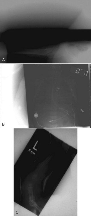
FIGURE 21-15 A sampling of histogram analysis errors. (Courtesy Barry Burns, University of North Carolina.)
Digital radiographic IPs now are available in the standard sizes shown in Box 21-1. The 14- × 17-inch image receptor is history; it has been replaced by a 35- × 43-cm image receptor.
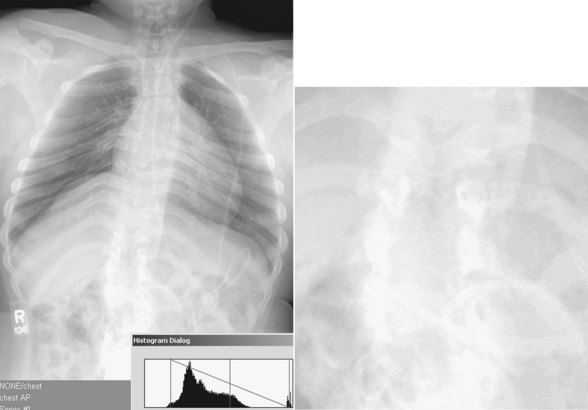
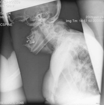
Collimation of the projected area x-ray beam is important for patient radiation dose reduction and for improved image contrast in screen-film radiography. In DR, proper collimation has the added value of defining the image histogram. If improperly collimated, the histogram can be improperly analyzed, resulting in an artifact such as that shown in Figure 21-16.
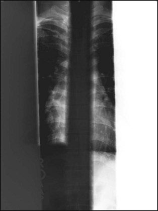
FIGURE 21-16 The blacked-out spine on this anteroposterior view was restored by engaging the automatic collimation feature. The white out on the patient’s left side was fixed by postconing that area and then engaging the “collimated image.” (Courtesy Dennis Bowman, Community Hospital of the Monterrey Peninsula.)
Digital image receptors normally can recognize even-numbered (i.e., two or four) x-ray exposure fields that are centered and cleanly collimated. Three on one and four on one are not recommended unless the unexposed portion is shielded. Figure 21-17 is a good example of reduced contrast when three on one is used.
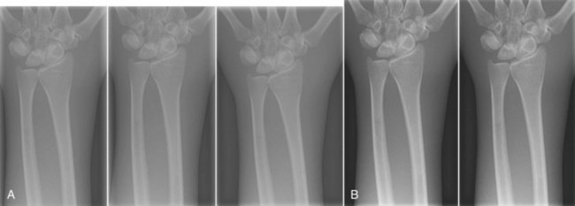
FIGURE 21-17 Loss of contrast is obvious when three on one versus two on one imaging is compared. (Courtesy Barry Burns, University of North Carolina.)
For the image histogram to be properly analyzed, each collimated field should consist of four distinct collimated margins, as seen in Figure 21-18. The use of three collimated margins usually works, but when fewer than three are used, artifacts may result.
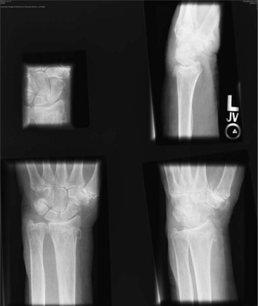
FIGURE 21-18 If all four wrist images have the same signal intensity, the radiographer changed technique appropriately. Technique was not properly adjusted for the oblique view in the lower right region. (Courtesy Dennis Bowman, Community Hospital of the Monterrey Peninsula.)
If images are not collimated and centered, image receptor exposure will not be accurate and cannot be used for image quality evaluation.
If multiple fields are projected onto a single IP, each must have clear, collimated edges and margins between each field. This process, called partitioning, allows two or more images to be projected on a single IP. Figure 21-19 illustrates the opposite situation.
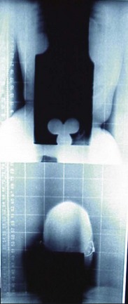
FIGURE 21-19 Two computed radiography plates used for spine imaging were placed into the processor in the wrong order. (Courtesy Barbara Smith Pruner, Portland Community College.)
Partitioning of multiple digital images on a single IP results in proper separation and collimation of each image.
The cause of these collimation artifacts is vendor algorithm related. The exposure field recognition algorithm is unable to match image histograms if the fields are not clear. This algorithm is based on edge detection or area detection. Further postprocessing of each image requires digital data representative of anatomy—not twice-irradiated or unirradiated portions of the IP.
Alignment
Alignment of the exposure field on the IP is important in the same way and for the same reason as collimation. When an image field, such as that shown in Figure 21-20, is not oriented with the size and dimensions of the IP, image artifacts can appear.
1. Define or otherwise identify the following:
2. What are the three general classifications of digital image artifacts?
3. What is the for-processing image, and how is it manipulated?
4. What does it mean when a single digital radiographic image is not properly aligned with the IP? Diagram such a situation.
5. What is the appearance of the radiation response curve for a digital radiographic image receptor?
6. Which digital imaging modality generates the largest image file, and approximately how large is it?
7. What is the difference between lossless and lossy compression?
8. Diagram improper margins of three digital images on a single IP.
9. How many distinct margins should appear on a digital radiograph?
10. Why is backscatter radiation important in DR?
11. What are the units on each axis of a digital radiographic image histogram?
12. What type of algorithm is used to correct for malfunctioning pixels?
13. Why is data compression often required for digital images?
14. What do the two outlying peaks on a digital image histogram represent?
15. What is the life expectancy of a CR IP?
16. Relate the tissues of a DR to position on the radiation response curve.
17. Why is it important for the radiologic technologist to select the proper imaging protocol for each digital imaging examination?
18. How does the heel effect appear on a digital image receptor?
19. Excessive compression can result in what form of image artifact?
20. Is an image histogram updated from time to time? If so, why?
The answers to the Challenge Questions can be found by logging on to our website at http://evolve.elsevier.com.