6 Hemodynamics
1. Define the relation between the velocity of blood flow and vascular cross-sectional area.
2. Describe the factors that govern the relationship between blood flow and pressure gradient.
3. Distinguish between resistances in series and resistances in parallel.
4. Distinguish between laminar flow and turbulent flow.
5. Describe the influence of the particulates in blood on blood flow.
The precise mathematical expression of the pulsatile flow of blood through the cardiovascular system remains to be solved. The heart is a complicated pump, and its behavior is affected by a variety of physical and chemical factors. The blood vessels are multibranched, elastic conduits of continuously varying dimensions. The blood itself is not a simple, homogeneous solution but is instead a complex suspension of red and white corpuscles, platelets, and lipid globules dispersed in a colloidal solution of proteins.
Despite these complex factors, considerable insight may be gained from an understanding of the elementary principles of fluid mechanics as they pertain to simple physical systems. Such principles are elaborated in this chapter to explain the interrelationships among the blood flow, the blood pressure, and the dimensions of the various components of the systemic circulation.
Velocity of the Bloodstream Depends on Blood Flow and Vascular Area
In describing the variations in blood flow in different vessels, the terms velocity and flow must first be distinguished. The former term, sometimes designated as linear velocity, means the rate of displacement with respect to time and it has the dimensions of distance per unit time, for example, cm/s. The flow, often designated as volume flow, has the dimensions of volume per unit time, for example, cm3/s. In a conduit of varying cross-sectional dimensions, velocity, v, flow, Q, and cross-sectional area, A, are related by the following equation:
 (1)
(1)The interrelationships among velocity, flow, and area are portrayed in Figure 6-1. The flow of an incompressible fluid past successive cross-sections of a rigid tube must be constant. For a given constant flow, the velocity varies inversely as the cross-sectional area (see Figure 1-3). Thus for the same volume of fluid per second passing from section a into section b, where the cross-sectional area is five times greater, the velocity diminishes to one fifth of its previous value. Conversely, when the fluid proceeds from section b to section c, where the cross-sectional area is one tenth as great, the velocity of each particle of fluid must increase tenfold.
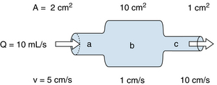
FIGURE 6-1 As fluid flows through a tube of variable cross-sectional area, A, the linear velocity, v, varies inversely with the cross-sectional area.
The velocity at any point in the system depends not only on the cross-sectional area but also on the flow, Q. This in turn depends on the pressure gradient, properties of the fluid, and dimensions of the entire hydraulic system, as discussed in the next section. For any given flow, however, the ratio of the velocity past one cross-section relative to that past a second cross-section depends only on the inverse ratio of the respective areas; that is,
 (2)
(2)This rule pertains regardless of whether a given cross-sectional area applies to a system that consists of a single large tube or to a system made up of several smaller tubes in parallel.
As shown in Figure 1-3, velocity decreases progressively as the blood traverses the aorta, its larger primary branches, the smaller secondary branches, and the arterioles. Finally, a minimal value is reached in the capillaries. As the blood then passes through the venules and continues centrally toward the venae cavae, the velocity progressively increases again. The relative velocities in the various components of the circulatory system are related only to the respective cross-sectional areas. Thus each point on the cross-sectional area curve is inversely proportional to the corresponding point on the velocity curve (see Figure 1-3).
Blood Flow Depends on the Pressure Gradient
In that portion of a hydraulic system in which the total energy remains virtually constant, changes in velocity may be accompanied by appreciable alterations in the measured pressure. Consider three sections (A, B, and C) of the hydraulic system depicted in Figure 6-2. Six pressure probes, or Pitot tubes, have been inserted. The openings of three of these (2, 4, and 6) are tangential to the direction of flow and hence measure the lateral, or static, pressure within the tube. The openings of the remaining three Pitot tubes (1, 3, and 5) face upstream. Therefore they detect the total pressure, which is the lateral pressure plus a dynamic pressure component that reflects the kinetic energy of the flowing fluid. This dynamic component, Pdyn, of the total pressure may be calculated from the following equation:
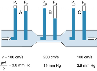
FIGURE 6-2 In a narrow section, B, of a tube, the linear velocity, v, and hence the dynamic component of pressure, ρv2/2, are greater than in the wide sections, A and C, of the same tube. If the total energy is virtually constant throughout the tube (i.e., if the energy loss due to viscosity is negligible), the total pressures (P1, P3, and P5) are not detectably different, but the lateral pressure, P4, in the narrow section is less than the lateral pressures (P2 and P6) in the wide sections of the tube.
 (3)
(3)where ρ is the density of the fluid and v is the velocity. If the midpoints of segments A, B, and C are at the same hydrostatic level, the corresponding total pressures, P1, P3, and P5, will be equal, provided that the energy loss from viscosity in these segments is negligible. However, because of the changes in cross-sectional area, the concomitant velocity changes alter the dynamic component.
In sections A and C, let ρ = 1 g/cm3 and v = 100 cm/s. From equation 3:
because 1330 dynes/cm2 = 1 mm Hg. In the narrow section, B, let the velocity be twice as great as in sections A and C. Therefore:
Hence in the wide sections of the conduit, the lateral pressures (P2 and P6) will be only 3.8 mm Hg less than the respective total pressures (P1 and P5), whereas in the narrow section, the lateral pressure (P4) is 15 mm Hg less than the total pressure (P3).
The peak velocity of flow in the ascending aorta of normal dogs is about 150 cm/second (s). Therefore the measured pressure at this site may vary significantly, depending on the orientation of the pressure probe. In the descending thoracic aorta the peak velocity is substantially less than that in the ascending aorta (Figure 6-3), and lesser velocities have been recorded in still more distal arterial sites. In most arterial locations the dynamic component is a negligible fraction of the total pressure, and the orientation of the pressure probe does not materially influence the pressure recorded. At the site of a constriction, however, the dynamic pressure component may attain substantial values. In aortic stenosis, for example, the entire output of the left ventricle is ejected through a narrow aortic valve orifice. The high flow velocity is associated with a large kinetic energy, and therefore the lateral pressure is correspondingly reduced.
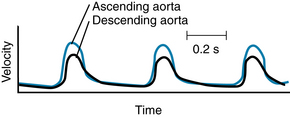
FIGURE 6-3 Velocity of the blood in the ascending and descending aorta of a dog.
(Redrawn from Falsetti HL, Kiser KM, Francis GP, et al: Sequential velocity development in the ascending and descending aorta of the dog. Circ Res 31:328, 1972.)
CLINICAL BOX
The pressure tracings shown in Figure 6-4 were obtained from two pressure transducers inserted into the left ventricle of a patient with aortic stenosis. The transducers were located on the same catheter and were 5 cm apart. When both transducers were well within the left ventricular cavity (Figure 6-4A), they both recorded the same pressures. However, when the proximal transducer was positioned in the aortic valve orifice (Figure 6-4B), the lateral pressure recorded during ejection was much less than that recorded by the transducer in the ventricular cavity. This pressure difference was associated almost entirely with the much greater velocity of flow in the narrowed valve orifice than in the ventricular cavity. The pressure difference reflects mainly the conversion of some potential energy to kinetic energy. When the catheter was withdrawn still farther, so that the proximal transducer was in the aorta (Figure 6-4C), the pressure difference was even more pronounced, because substantial energy was lost through friction (viscosity) as blood flowed rapidly through the narrow aortic valve.
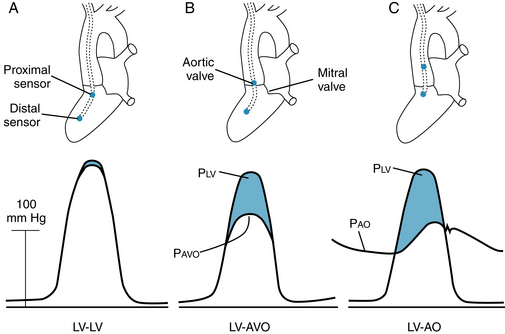
FIGURE 6-4 Pressures (P) recorded by two transducers in a patient with aortic stenosis. A, Both transducers were in the left ventricle (LV-LV). B, One transducer was in the left ventricle and the other was in the aortic valve orifice (LV-AVO). C, One transducer was in the left ventricle and the other was in the ascending aorta (LV-AO). Pao, pressure in ascending aorta; Pavo, aortic valve orifice; Plv, pressure in left ventricle.
(Redrawn from Pasipoularides A, Murgo JP, Bird JJ, et al: Fluid dynamics of aortic stenosis: mechanisms for the presence of subvalvular pressure gradients. Am J Physiol 246:H542, 1984.)
The reduction of lateral pressure in the region of the stenotic valve orifice influences coronary blood flow in patients with aortic stenosis. The orifices of the right and left coronary arteries are located in the sinuses of Valsalva, just behind the valve leaflets. The initial segments of these vessels are oriented at right angles to the direction of blood flow through the aortic valves. Therefore the lateral pressure is that component of total pressure that propels the blood through the two major coronary arteries. During the ejection phase of the cardiac cycle, the lateral pressure is diminished by the conversion of potential energy to kinetic energy. This process is greatly exaggerated in aortic stenosis because of the high flow velocities.
Relationship between Pressure and Flow Depends on the Characteristics of the Conduits
The most fundamental law that governs the flow of fluids through cylindrical tubes was derived empirically by the French physiologist Jean Poiseuille. He was primarily interested in the physical determinants of blood flow, but he replaced blood with simpler liquids for his measurements of flow through glass capillary tubes. His work was so precise and important that his observations have been designated Poiseuille’s law. Subsequently, this same law has been derived theoretically.
Poiseuille’s law is applicable to the flow of fluids through cylindrical tubes only under special conditions, namely, in the case of steady, laminar flow of newtonian fluids. The term steady flow signifies the absence of variations of flow in time, that is, a nonpulsatile flow. Laminar flow is the type of motion in which the fluid moves as a series of individual layers, with each stratum moving at a different velocity from its neighboring layers (Figure 6-5). In the case of flow through a tube, the fluid consists of a series of infinitesimally thin concentric tubes sliding past one another. Laminar flow is described in greater detail later, where it is distinguished from turbulent flow. Also, a newtonian fluid is defined more precisely. For the present discussion, it may be considered to be a homogeneous fluid, such as water, in contradistinction to a suspension, such as blood.
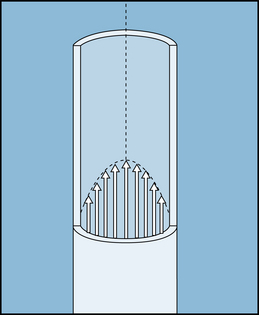
FIGURE 6-5 In laminar flow, all elements of the fluid move in streamlines that are parallel to the axis of the tube; movement does not occur in a radial or circumferential direction. The layer of fluid in contact with the wall is motionless; the fluid that moves along the axis of the tube has the maximal velocity.
Pressure is one of the principal determinants of the rate of flow. The pressure, P, in dynes/cm2, at a distance h, in centimeters, below the surface of a liquid is:
 (4)
(4)where ρ is the density of the liquid in g/cm3 and g is the acceleration of gravity in cm/s2. For convenience, however, pressure is frequently expressed simply in terms of the height of the column of liquid above some arbitrary reference point.
Consider the tube connecting reservoirs R1 and R2 in Figure 6-6A. Let reservoir R1 be filled with liquid to height h1, and let reservoir R2 be empty, as in Figure 6-6A. The outflow pressure, Po, is therefore equal to the atmospheric pressure, which shall be designated as the zero, or reference, level. The inflow pressure, Pi, is then equal to the same reference level plus the height, h1, of the column of liquid in reservoir R1. Under these conditions, let the flow, Q, through the tube be 5 mL/s.
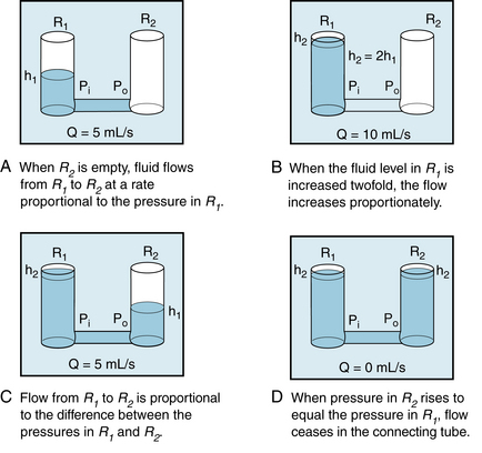
FIGURE 6-6 A to D, The flow, Q, of fluid through a tube connecting two reservoirs, R1 and R2, is proportional to the difference between the pressure at the inflow end (Pi) and the pressure at the outflow end (Po) of the tube. h1 and h2, heights of liquid in the reservoir.
If reservoir R1 is filled to height h2, which is twice h1, and reservoir R2 is again empty (as in panel B), the flow is twice as great, that is, 10 mL/s. Thus with reservoir R2 empty, the flow is directly proportional to the inflow pressure, Pi.
If reservoir R2 is now allowed to fill to height h1, and the fluid level in R1 is maintained at h2 (as in panel C), the flow again becomes 5 mL/s. Thus, flow is directly proportional to the difference between inflow and outflow pressures:
 (5)
(5)If the fluid level in R2 attains the same height as in R1, flow ceases (panel D).
For any given pressure difference between the two ends of a tube, the flow depends on the dimensions of the tube. Consider the tube connected to the reservoir in Figure 6-7A. With length l1 and radius r1, the flow Q1 is observed to be 10 mL/s.
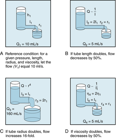
FIGURE 6-7 A to D, The flow, Q, of fluid through a tube is inversely proportional to the length, l, and the viscosity, η, and is directly proportional to the fourth power of the radius, r. h1 and h2, heights of liquid in the reservoir.
The tube connected to the reservoir in panel B has the same radius but is twice as long. Under those conditions the flow Q2 is found to be 5 mL/s, or only half as great as Q1. Conversely, for a tube half as long as l1, the flow would be twice as great as Q1. In other words, flow is inversely proportional to the length of the tube:
 (6)
(6)The tube connected to the reservoir in Figure 6-7C is the same length as l1, but the radius is twice as great. Under these conditions, the flow Q3 is found to increase to a value of 160 mL/s, which is 16 times greater than Q1. The precise measurements of Poiseuille revealed that flow varies directly as the fourth power of the radius:
 (7)
(7)Because r3 = 2r1 in the example above (Figure 6-7C), Q3 will be proportional to (2r1)4, or  ; therefore Q3 will equal 16Q1.
Finally, for a given pressure difference and for a cylindrical tube of given dimensions, the flow varies as a function of the nature of the fluid itself. This flow-determining property of fluids is termed viscosity, η, which Newton defined as the ratio of shear stress to the shear rate of the fluid. Those fluids for which the shear rate is proportional to the shear stress are known as newtonian fluids. If the shear rate is not proportional to the shear stress, the fluid is nonnewtonian.
These terms may be comprehended more clearly if one considers the flow of a homogeneous fluid between parallel plates. In Figure 6-8, let the bottom plate (the bottom of a large basin) be stationary, and let the upper plate move at a constant velocity along the upper surface of the fluid. The shear stress, η, is defined as the ratio of F:A, where F is the force applied to the upper plate in the direction of its motion along the upper surface of the fluid, and A is the area of the upper plate in contact with the fluid. The shear rate is du/dy, where u is the velocity of a minute element of the fluid in the direction parallel to the motion of the upper plate, and y is the distance of that fluid element above the bottom, stationary plate.
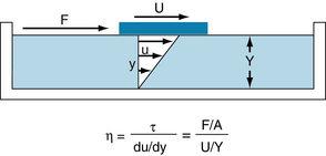
FIGURE 6-8 For a newtonian fluid, the viscosity, η, is defined as the ratio of shear stress, τ, to shear rate, du/dy. For a plate of contact area, A, moving across the surface of a liquid, τ equals the ratio of the force, F, applied in the direction of motion to the contact area, and du/dy equals the ratio of the velocity of the plate, U, to the depth of the liquid, Y.
For a movable plate traveling at constant velocity across the surface of a homogeneous fluid, the velocity profile of the fluid will be linear. The fluid layer in contact with the upper plate will adhere to it and therefore will move at the same velocity, U, as the plate. Each minute element of fluid between the plates will move at a velocity, u, proportional to its distance, y, from the lower plate. Therefore the shear rate will be U/Y, where Y is the total distance between the two plates. Because viscosity, η, is defined as the ratio of shear stress, τ, to the shear rate, du/dy, in the example illustrated in Figure 6-8:
 (8)
(8)Thus the dimensions of viscosity are dynes/cm2 divided by (cm/s)/cm, or dynes•s/cm2. In honor of Poiseuille, 1 dyne•s/cm2 has been termed a poise. The viscosity of water at 20° C is approximately 0.01 poise, or 1 centipoise.
With regard to the flow of newtonian fluids through cylindrical tubes, the flow varies inversely as the viscosity. Thus in the example of flow from the reservoir in Figure 6-7D, if the viscosity of the fluid in the reservoir were doubled, the flow would be halved (5 mL/s instead of 10 mL/s).
In summary, for the steady, laminar flow of a newtonian fluid through a cylindrical tube, the flow, Q, varies directly as the pressure difference, Pi − Po, and the fourth power of the radius, r, of the tube, and it varies inversely as the length, l, of the tube and the viscosity, η, of the fluid. The full statement of Poiseuille’s law is
 (9)
(9)where π/8 is the constant of proportionality.
Resistance to Flow
In electrical theory the resistance, R, is defined as the ratio of voltage drop, E, to current flow, I. Similarly, in fluid mechanics the hydraulic resistance, R, may be defined as the ratio of pressure drop, Pi − Po, to flow, Q; Pi and Po are the pressures at the inflow and outflow ends, respectively, of the hydraulic system. For the steady, laminar flow of a newtonian fluid through a cylindrical tube, the physical components of hydraulic resistance may be appreciated by rearranging Poiseuille’s law to give the hydraulic resistance equation:
 (10)
(10)Thus when Poiseuille’s law applies, the resistance to flow depends only on the dimensions of the tube and on the characteristics of the fluid.
The principal determinant of the resistance to blood flow through any vessel within the circulatory system is its caliber because resistance varies with the fourth power of the tube radius. The resistance to flow through small blood vessels in cat mesentery has been measured, and the resistance per unit length of vessel (R/l) is plotted against the vessel diameter in Figure 6-9. The resistance is highest in the capillaries (diameter 7 µm), and it diminishes as the vessels increase in diameter on the arterial and venous sides of the capillaries. The values of R/l were found to be virtually proportional to the fourth power of the diameter (or radius) for the larger vessels on both sides of the capillaries.
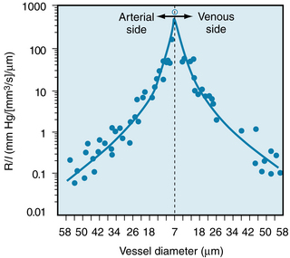
FIGURE 6-9 The resistance per unit length (R/l) for individual small blood vessels in the cat mesentery. The capillaries, diameter 7 µm, are denoted by the vertical dashed line. Resistances of the arterioles are plotted to the left and resistances of the venules are plotted to the right of that line. The solid circles represent the actual data. The two curves through the data represent the following regression equations for the arteriole and venule data, respectively: arterioles, R/l = 1.02 × 10⁶D−4.04, and venules, R/l = 1.07 × 10⁶D−3.94. Note that for both types of vessels, the resistance per unit length is inversely proportional to the fourth power (within 1%) of the vessel diameter.
(Redrawn from Lipowsky HH, Kovalcheck S, Zweifach BW: The distribution of blood rheological parameters in the microvasculature of cat mesentery. Circ Res 43:738, 1978.)
Figure 1-3 shows that the greatest upstream to downstream drop in internal pressure occurs in the arterioles and small arteries. It follows that the greatest resistance to flow resides in the arterioles because the total flow is the same through the various series components of the circulatory system. For example, if Ra represents the resistance of the arterioles, and Rx represents the resistance of any other component of the vascular system in series with the arterioles, then by the definition of hydraulic resistance (equation 10),
 (11)
(11)for the arterioles, and
 (12)
(12)for the other vascular component.
However, the two components are in series, Qa = Qx, as stated previously. Therefore:
 (13)
(13)That is, the ratio of the pressure drop across the length of the arterioles to the pressure drop across the length of any other series component of the vascular system is equal to the ratio of the hydraulic resistances of these two vascular components.
The reason that the highest resistance does not reside in the capillaries (as might otherwise be suspected from Figure 6-9) is related to the relative numbers of parallel capillaries and parallel arterioles, as explained later (see Figure 6-11). The arterioles are vested with a thick coat of circularly arranged smooth muscle fibers, by means of which the lumen radius may be varied. From the hydraulic resistance equation, wherein R varies inversely with r4, it is clear that small changes in radius will alter resistance greatly.
Resistances in Series and in Parallel
In the cardiovascular system, the various types of vessels listed along the horizontal axis in Figure 1-3 lie in series with one another. For two vessels arranged in series, a red blood cell that flows through the upstream vessel will also flow through the downstream vessel. Furthermore, the individual members of a given category of vessels are ordinarily arranged in parallel with one another (see Figure 1-1). For two vessels arranged in parallel, a red blood cell will pass through one of these vessels but not through the other during one circuit around the body. For example, the capillaries throughout the body are in most instances parallel elements. However, notable exceptions are the renal vasculature (wherein the peritubular capillaries are in series with the glomerular capillaries) and the splanchnic vasculature (wherein the intestinal and hepatic capillaries are aligned in series). Formulas for the total hydraulic resistance of tubes arranged in series and in parallel have been derived in the same manner as those for similar combinations of electrical resistances.
Three hydraulic resistances, R1, R2, and R3, are arranged in series in the schema depicted in Figure 6-10. The pressure drop across the entire system—that is, the difference between inflow pressure, Pi, and outflow pressure, Po—consists of the sum of the pressure drops across each of the individual resistances (equation a in Figure 6-10). Under steady-state conditions, the flow, Q, through any given cross-section must equal the flow through any other cross-section. When each component in equation a is divided by Q (equation b), it becomes evident from the definition of resistance (equation c) that the total resistance, Rt, of the entire system of tubes in series equals the sum of the individual resistances: that is,
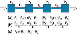
FIGURE 6-10 For resistances (R1, R2, and R3) arranged in series, the total resistance, Rt, equals the sum of the individual resistances.
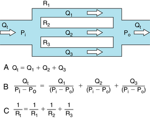
FIGURE 6-11 For resistances (R1, R2, and R3) arranged in parallel, the reciprocal of the total resistance, Rt, equals the sum of the reciprocals of the individual resistances.
 (14)
(14)For resistances in parallel, as illustrated in Figure 6-11, the inflow and outflow pressures are the same for all tubes. Under steady-state conditions, the total flow, Qt, through the system equals the sum of the flows through the individual parallel elements (equation a in Figure 6-10). Because the pressure gradient (Pi − Po) is identical for all parallel elements, each term in equation a may be divided by that pressure gradient to yield equation b. From the definition of resistance, equation c may be derived. This equation states that the reciprocal of the total resistance, Rt, of tubes in parallel equals the sum of the reciprocals of the individual resistances; that is,
 (15)
(15)Stated in another way, if we define hydraulic conductance as the reciprocal of resistance, it becomes evident that, for tubes in parallel, the total conductance is the sum of the individual conductances.
Considering a few simple illustrations helps some of the fundamental properties of parallel hydraulic systems become apparent. For example, if the resistance of the three parallel elements in Figure 6-11 were all equal, then
 (16)
(16) (17)
(17)and
 (18)
(18)Thus the total resistance is less than any of the individual resistances. Furthermore, it becomes evident that for any parallel arrangement, the total resistance must be less than that of any individual component. For example, consider a system in which a very high-resistance tube is added in parallel to a low-resistance tube. The total resistance must be less than that of the low-resistance component by itself, because the high-resistance component affords an additional pathway, or conductance, for fluid flow.
Flow may be Laminar or Turbulent
Under certain conditions, the flow of a fluid in a cylindrical tube is laminar (sometimes called streamlined), as illustrated in Figure 6-5. The thin layer of fluid in contact with the wall of the tube adheres to the wall and thus is motionless. The layer of fluid just central to this external lamina must shear against this motionless layer and therefore moves slowly, but with a finite velocity. Similarly, the adjacent, more central layer travels still more rapidly. The longitudinal velocity profile is that of a paraboloid (see Figure 6-5). The velocity of the fluid adjacent to the wall is zero, whereas the velocity at the center of the stream is maximum and equal to twice the mean velocity of flow across the entire cross-section of the tube. In laminar flow, fluid elements remain in one lamina, or streamline, as the fluid progresses longitudinally along the tube.
Irregular motions of the fluid elements may develop in the flow of fluid through a tube; this flow is called turbulent. Under such conditions, fluid elements do not remain confined to definite laminae, but rapid, radial mixing occurs (Figure 6-12). A much greater pressure is required to force a given flow of fluid through the same tube when the flow is turbulent than when it is laminar. In turbulent flow the pressure drop is approximately proportional to the square of the flow rate, whereas in laminar flow the pressure drop is proportional to the first power of the flow rate. Hence to produce a given flow, a pump such as the heart must do considerably more work to generate a given flow if turbulence develops.
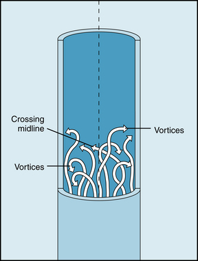
FIGURE 6-12 In turbulent flow the elements of the fluid move irregularly in axial, radial, and circumferential directions. Vortices frequently develop.
Whether turbulent or laminar flow will exist in a tube under given conditions may be predicted on the basis of a dimensionless number called the Reynold number, NR. This number represents the ratio of inertial to viscous forces. For a fluid flowing through a cylindric tube,
 (19)
(19)where D is the tube diameter,  is the mean velocity, ρ is the density, and η is the viscosity. For NR = 2000, the flow is usually laminar; for NR > 3000, the flow is turbulent. Various possible conditions may develop in the transition range of NR between 2000 and 3000. The definition of NR indicates that large diameters, high velocities, and low viscosities predispose to turbulence because flow tends to be laminar at low NR and turbulent at high NR
Turbulence is usually accompanied by audible vibrations. When turbulent flow exists within the cardiovascular system, it is usually detected as a murmur. The factors listed previously that predispose to turbulence may account for murmurs heard clinically. In severe anemia, functional cardiac murmurs (murmurs not caused by structural abnormalities) are frequently detectable. The physical basis for such murmurs resides in (1) the reduced viscosity of blood in anemia and (2) the high flow velocities associated with the high cardiac output that usually prevails in anemic patients. Turbulence also occurs when the cross-sectional area of the bloodstream suddenly changes, as when the blood passes through a narrowed (stenotic) cardiac valve or when it passes through an abnormal widening (aneurysm) of a large artery. Such abrupt changes in dimensions of the bloodstream cause audible murmurs.
Blood clots, or thrombi, are much more likely to develop in turbulent than in laminar flow. One of the problems with the use of artificial valves in the surgical treatment of valvular heart disease is that thrombi may occur in association with the prosthetic valve. The thrombi may be dislodged and occlude a crucial artery. It is thus important to design such valves to avert turbulence.
Shear Stress on the Vessel Wall
In Figure 6-8, an external force is applied to a plate floating on the surface of a liquid in a large basin. This force, exerted parallel to the surface, causes a shearing stress on the liquid below and thereby produces a differential motion of each layer of liquid relative to the adjacent layers. At the bottom of the basin, the flowing liquid exerts a shearing stress on the surface of the basin in contact with the liquid. If the equation for viscosity stated in Figure 6-8 is rearranged, it is apparent that the shear stress, τ, equals η (du/dy); that is, the shear stress equals the product of the viscosity and the shear rate. Hence the greater the rate of flow, the greater the shear stress that the liquid exerts on the walls of the container in which it flows.
For precisely the same reasons, the rapidly flowing blood in a large artery tends to pull the endothelial lining of the artery along with it. This force (viscous drag) is proportional to the shear rate (du/dy) of the layers of blood very close to the wall. For a flow regimen that obeys Poiseuille’s law,
 (20)
(20)The greater the rate of blood flow (Q) in the artery, the greater will be du/dy near the arterial wall, and the greater will be the viscous drag (τ). Under physiological conditions, shear stress is 1 to 6 dynes/cm2 in veins and 10 to 70 dynes/cm2 in arteries. Also, shear stress is linked to biochemical changes in blood vessel function. Thus, laminar flow with high shear can protect against atherosclerosis by reducing the synthesis of atherogenic genes and increasing the production of atheroprotective genes. Turbulent flow patterns, seen at vessel bifurcations and curvatures, are likely to increase synthesis of genes that promote inflammation, the cause of atherosclerotic plaque formation. For example, angiotensin II, an endogenous substance, is implicated in inflammation that underlies atherosclerosis. Physiological shear stress may be atherprotective by causing a reduction (downregulation) of angiotensin type 1 receptors (AT1Rs) on the surface of endothelial cells.
CLINICAL BOX
In certain types of arterial disease, particularly in patients with hypertension, the subendothelial layers tend to degenerate locally, and small regions of the endothelium may lose their normal support. The viscous drag on the arterial wall may cause a tear between a normally supported region and an unsupported region of the endothelial lining. Blood may then flow from the vessel lumen through the rift in the lining and dissect between the various layers of the artery. Such a lesion is called a dissecting aneurysm. It occurs most commonly in the proximal portions of the aorta and is extremely serious. One reason for its predilection for this site is the high velocity of blood flow, with the associated large values of du/dy at the endothelial wall. The shear stress at the vessel wall also influences many other vascular functions, such as the permeability of the vascular walls to large molecules, the biosynthetic activity of the endothelial cells, the integrity of the formed elements in the blood, and the coagulation of the blood.
Rheologic Properties of Blood
The viscosity of a newtonian fluid, such as water, may be determined by measuring the rate of flow of the fluid at a given pressure gradient through a cylindrical tube of known length and radius. As long as the fluid flow is laminar, the viscosity may be computed by substituting these values into Poiseuille’s equation. The viscosity of a given newtonian fluid at a specified temperature will be constant over a wide range of tube dimensions and flows. However, for a nonnewtonian fluid, the viscosity calculated by substituting into Poiseuille’s equation may vary considerably as a function of tube dimensions and flows. Therefore, the term viscosity does not have a unique meaning in considering the rheologic properties of a suspension such as blood. The terms anomalous viscosity and apparent viscosity are frequently applied to the value of viscosity obtained for blood under the particular conditions of measurement.
Rheologically, blood is a suspension of formed elements, principally erythrocytes, in a relatively homogeneous liquid, the blood plasma. For this reason, the apparent viscosity of blood varies as a function of the hematocrit ratio (ratio of volume of red blood cells to volume of whole blood). In Figure 6-13 the upper curve represents the ratio of the apparent viscosity of whole blood to that of plasma over a range of hematocrit ratios from 0% to 80%, measured in a tube 1 mm in diameter. The viscosity of plasma is 1.2 to 1.3 times that of water. Figure 6-13 (upper curve) shows that blood, with a normal hematocrit ratio of 45%, has an apparent viscosity 2.4 times that of plasma.
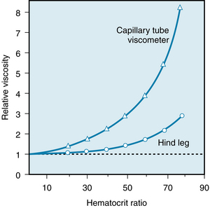
FIGURE 6-13 The viscosity of whole blood, relative to that of plasma, increases at a progressively greater rate as the hematocrit ratio increases. For any given hematocrit ratio, the apparent viscosity of blood is less when measured in a biological viscometer (such as the hind leg of a dog) than in a conventional capillary tube viscometer.
(Redrawn from Levy MN, Share L: The influence of erythrocyte concentration upon the pressure-flow relationships in the dog’s hind limb. Circ Res 1:247, 1953.)
For any given hematocrit ratio, the apparent viscosity of blood depends on the dimensions of the tube employed in estimating the viscosity. Figure 6-14 demonstrates that the apparent viscosity of blood diminishes progressively as tube diameter decreases below a value of about 0.3 mm. The diameters of the highest-resistance blood vessels, the arterioles, are considerably less than this critical value. This phenomenon therefore reduces the resistance to flow in the blood vessels that possess the greatest resistance.
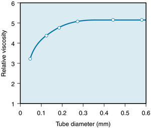
FIGURE 6-14 The viscosity of blood, relative to that of water, increases as a function of tube diameter up to a diameter of about 0.3 mm.
(Redrawn from Fähraeus R, Lindqvist T: The viscosity of the blood in narrow capillary tubes. Am J Physiol 96:562, 1931.)
CLINICAL BOX
In severe anemia, blood viscosity is low. With greater hematocrit ratios, the relative viscosity increases (see Figure 6-13). This effect is especially profound at the upper range of erythrocyte concentrations. A rise in hematocrit ratio from 45% to 70%, which occurs in polycythemia, increases the relative viscosity more than twofold, with a proportionate effect on the resistance to blood flow. The effect of such a change in hematocrit ratio on peripheral resistance may be appreciated when it is recognized that even in the most severe cases of essential hypertension, total peripheral resistance rarely increases by more than a factor of two. In essential hypertension, the increase in peripheral resistance is achieved by arteriolar vasoconstriction.
The apparent viscosity of blood, when measured in living tissues, is considerably less than when it is measured in a conventional capillary tube viscometer with a diameter greater than 0.3 mm. In the lower curve of Figure 6-13, the apparent viscosity of blood was assessed by using the hind leg of an anesthetized dog as a biological viscometer. Over the entire range of hematocrit ratios, the apparent viscosity was less when measured in the living tissue than in the capillary tube viscometer (upper curve), and the disparity was greater the higher the hematocrit ratio.
The influence of tube diameter on apparent viscosity depends in part on the change in actual composition of the blood as it flows through small tubes. The composition changes because the red blood cells tend to accumulate in the faster axial stream in the blood vessels, whereas the blood component that flows in the slower marginal layers is mainly plasma.
To illustrate this phenomenon, a reservoir such as R1 in Figure 6-6C has been filled with blood possessing a given hematocrit ratio. The blood in R1 was constantly agitated to prevent settling and was permitted to flow through a narrow capillary tube into reservoir R2. As long as the tube diameter was substantially greater than the diameter of the red blood cells, the hematocrit ratio of the blood in R2 was not detectably different from that in R1. Surprisingly, however, the hematocrit ratio of the blood contained within the tube was found to be considerably lower than the hematocrit ratio of the blood in either reservoir.
In Figure 6-15, the relative hematocrit is the ratio of the hematocrit in the tube to that in the reservoir at either end of the tube. For tubes of 300 µm diameter or greater, the relative hematocrit ratio was close to 1. However, as the tube diameter was reduced below 300 µm, the relative hematocrit ratio progressively diminished; for a tube diameter of 30 µm, the relative hematocrit ratio was only 0.65.
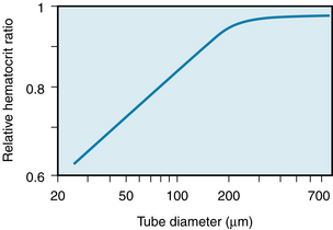
FIGURE 6-15 The relative hematocrit ratio of blood flowing from a feed reservoir through capillary tubes of various calibers, as a function of the tube diameter. The relative hematocrit is the ratio of the hematocrit of the blood in the tubes to that of the blood in the feed reservoir.
(Redrawn from Barbee JH, Cokelet GR: The Fahraeus effect. Microvasc Res 3:6, 1971.)
This effect, called the Fahraeus-Lindqvist phenomenon, results from a disparity in the relative velocities of the red blood cells and plasma. The red blood cells tend to traverse the tube in less time than the plasma because the axial portions of the bloodstream contain a greater proportion of red blood cells and move with a greater velocity. Measurement of transit times through various organs has shown that red blood cells do travel faster than the plasma. Furthermore, the hematocrit ratios of the blood contained in the smallest vessels in various tissues are lower than those in blood samples withdrawn from large arteries or veins in the same animal (Figure 6-16).
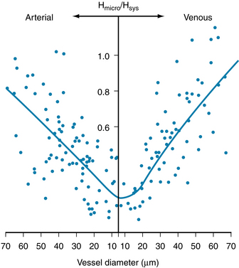
FIGURE 6-16 The hematocrit ratio (Hmicro) of the blood in various-sized arterial and venous microvessels in the cat mesentery, relative to the hematocrit ratio (Hsys) in the large systemic vessels. The hematocrit ratio is least in the capillaries and tiny venules.
(Modified from Lipowsky HH, Usami S, Chien S: In vivo measurements of “apparent viscosity” and microvessel hematocrit in the mesentery of the cat. Microvasc Res 19:297, 1980.)
The physical forces causing the drift of the erythrocytes toward the axial stream and away from the vessel walls are not fully understood. One factor is the great flexibility of the red blood cells. At low flow (or shear) rates, comparable with those in the microcirculation, flexible particles migrate toward the axis of a tube, whereas rigid particles do not. The concentration of flexible particles near the tube axis is enhanced by an increase in the shear rate.
The apparent viscosity of blood diminishes as the shear rate is increased (Figure 6-17), a phenomenon called shear thinning. The greater tendency of the erythrocytes to accumulate in the axial laminae at higher flow rates is partly responsible for this nonnewtonian behavior. However, a more important factor is that at very slow rates of shear, the suspended cells tend to form aggregates, which would increase viscosity. As the flow is increased, this aggregation would decrease and so would the apparent viscosity (see Figure 6-17).
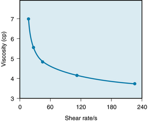
FIGURE 6-17 Decrease in the viscosity of blood (in centipoise) at increasing rates of shear. The shear rate refers to the velocity of one layer of fluid relative to that of the adjacent layers and is directionally related to the rate of flow.
(Redrawn from Amin TM, Sirs JA: The blood rheology of man and various animal species. Q J Exp Physiol 70:37, 1985.)
The tendency for the erythrocytes to aggregate at low flows depends on the concentration in the plasma of the larger protein molecules, especially fibrinogen. For this reason, the changes in blood viscosity with shear rate are much more pronounced when the concentration of fibrinogen is high. Also, at low flow rates, leukocytes tend to adhere to the endothelial cells of the microvessels and thereby increase the apparent viscosity.
The deformability of erythrocytes is also a factor in shear thinning, especially at high hematocrit ratios. The mean diameter of human red blood cells is about 8 µm, yet they are able to pass through openings with a diameter of only 3 µm. As blood that is densely packed with erythrocytes is made to flow at progressively greater rates, the erythrocytes become more and more deformed, diminishing the apparent viscosity of the blood. The flexibility of human erythrocytes is enhanced as the concentration of fibrinogen in the plasma increase (Figure 6-18).
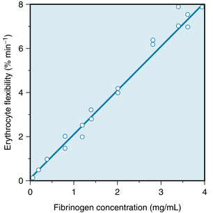
FIGURE 6-18 The effect of the plasma fibrinogen concentration on the flexibility of human erythrocytes.
(Redrawn from Amin TM, Sirs JA: The blood rheology of man and various animal species. Q J Exp Physiol 70:37, 1985.)
CLINICAL BOX
If the red blood cells become hardened, as they are in certain spherocytic anemias, shear thinning may become much less prominent. When erythrocytes are extremely deformed, especially in sickle cell anemia, they tend to aggregate and completely block flow in small vessels; the tissues supplied by those vessels frequently become infarcted.
Summary
 The vascular system is composed of two major subdivisions in series with each other—the systemic circulation and the pulmonary circulation.
Each subdivision consists of several types of vessels (e.g., arteries, arterioles, capillaries) aligned in series with one another. In general, the vessels of a given type are arranged in parallel with each other.
The mean velocity ( ) of blood flow in a given type of vessel is directly proportional to the total blood flow (Qt) being pumped by the heart, and it is inversely proportional to the cross-sectional area (A) of all the parallel vessels of that type; i.e.,
  .
.
The laterally directed pressure in the bloodstream decreases as the flow velocity increases; the decrement in lateral pressure is proportional to the square of the velocity.
When blood flow is steady and laminar in vessels larger than arterioles, the flow (Q) is proportional to the pressure drop down the vessel (Pi − Po) and to the fourth power of the radius (r), and it is inversely proportional to the length (l) of the vessel and to the viscosity (η) of the fluid; i.e., Q = π(Pi − Po)r4/8ηl (Poiseuille’s law).
For resistances aligned in series, the total resistance equals the sum of the individual resistances.
For resistances aligned in parallel, the reciprocal of the total resistance equals the sum of the reciprocals of the individual resistances.
Flow tends to become turbulent when flow velocity is high, when fluid viscosity is low, when tube diameter is large, or when the wall of the vessel is very irregular.
Blood flow is nonnewtonian in very small vessels; i.e., Poiseuille’s law is not applicable. The apparent viscosity of blood diminishes as shear rate (flow) increases and as the tube dimensions decrease.
Baskurt O.K., Meiselman H.J. Blood rheology and hemodynamics. Semin Thromb Hemost. 2003;29:435.
Cecchi E., Gigioli C., Valente S., et al. Role of hemodynamic shear stress in cardiovascular disease. Atheroclerosis. 2011;214:249.
Chiu J.-J., Chien S. Effects of disturbed flow on vascular endothelium: pathophysiological basis and clinical perspectives. Physiol Rev. 2011;91:327.
Helmke B.P. Molecular control of cytoskeletal mechanics by hemodynamic forces. Physiology. 2005;20:43.
Hoeks A.P.G., Samijo S.K., Brands P.J., et al. Noninvasive determination of shear-rate distribution across the arterial wall. Hypertension. 1995;26:26.
Kwaan H.C., Wang J. Hyperviscosity in polycythemia vera and other red cell abnormalities. Semin Thromb Hemost. 2003;29:451.
Long D.S., Smith M.L., Pries A., et al. Microviscometry reveals reduced blood viscosity and altered shear rate and shear stress profiles in microvessels after hemodilution. Proc Natl Acad Sci U S A. 2004;101:10060.
McCue S., Noria S., Langille B.L. Shear-induced reorganization of endothelial cell cytoskeleton and adhesion complexes. Trends Cardiovasc Med. 2004;14:143.
Pries A.R., Secomb T.W. Microvascular blood viscosity in vivo and the endothelial surface layer. Am J Physiol. 2005;289:H2657.
Pries A.R., Secomb T.W., Gaetgens P. Design principles of vascular beds. Circ Res. 1995;77:1017.
Resnick N., Yahav H., Shay-Salit A., et al. Fluid shear stress and the vascular endothelium: for better and for worse. Prog Biophys Mol Biol. 2003;81:177.
Tyml K., Anderson D., Lidington D., Ladak H.M. A new method for assessing arteriolar diameter and hemodynamic resistance using image analysis of vessel lumen. Am J Physiol. 2003;284:H1721.
CASE 6-6
History
A 70-year-old man complained of severe pain in his right leg whenever he walked briskly; the pain disappeared soon after he stopped walking. His doctor referred him to a vascular surgeon, who carried out several hemodynamic tests. Angiography showed partial obstruction by large arteriosclerotic plaques about 3 cm distal to the origin of the right femoral artery. The left femoral artery appeared to be normal. The mean arterial pressure in the left femoral artery with the patient at rest was 100 mm Hg, and the blood flow in this artery was 500 mL/min. The mean arterial pressure in the right femoral artery proximal to the obstruction was 100 mm Hg, and just distal to the obstruction, it was 80 mm Hg. The blood flow in this artery was 300 mL/min. The mean venous pressure was 10 mm Hg in the left and right femoral veins.
Questions
1. The resistance to blood flow in the vascular bed perfused by the right femoral artery was:
2. The resistance to blood flow (Rt) in the combined vascular beds perfused by both femoral arteries was:
3. The resistance to flow imposed by the arteriosclerotic obstruction in the right femoral artery amounted to: