Since its introduction in the early 1970s, computed tomography (CT) has played a significant role in the detection and management of human diseases in medicine. The technical evolution of CT has been dynamic, ranging from the first-generation single-slice “stop-and-go” technique to multislice volume scanning. The growth of volume CT scanners continues at a rapid rate, from 16- to 64-slice systems to the more recent 320-slice CT scanner. These developments have created a wide variety of clinical applications such as CT colonography, cardiac CT imaging, and CT screening (Brenner, 2006), for example. Furthermore, there has been an increase in CT use worldwide (Amis et al, 2007; Lee et al, 2007; Mukundan et al, 2007). For example, in the United States alone it has been estimated that the number of CT scans increased from 40 million in 2000 to 65 million in 2004 and it is expected to increase to 100 million in 2010 (Baker and Tilak, 2007). In association with the expanding use of CT in medicine, one other major concern that is receiving increasing attention in the literature relates to the potential for high radiation doses delivered by CT scanners (Amis et al, 2007; Baker and Tilak, 2007; Cody and McNitt-Gray, 2006; Colang et al, 2007; ECRI, 2007; Frush, 2006; Goodman and Brink, 2006; Martin and Semelka 2007; Moore et al, 2006; Siegel, 2006), and the potential risks of CT scanning (Brenner and Elliston, 2004; Brenner and Hall, 2007; Brenner et al, 2001; Wise, 2003).

With this in mind, all individuals working in CT, such as radiologists, technologists, medical physicists, physicians and manufacturers alike, should ask themselves three central questions: Why are the doses in CT so high? What is the dose to the patient at my institution? What can be done to reduce the high exposures in CT to protect both patients and personnel?

There are several reasons why these questions are important, as mentioned previously; however, perhaps the most important reason for understanding radiation dose in CT relates to the radiation risks (Brenner, 2006; Huda and Vance, 2007). In this regard, the dose for a CT examination may have to be estimated to make decisions regarding the benefits versus the risks of the procedure. CT manufacturers are now required by law to provide a dose table that shows the doses delivered to patients from their CT scanners.

The purpose of this chapter is to outline the fundamental concepts of radiation dose in CT. In particular, topics such as radiation quantities and their units, factors affecting dose in CT, CT dosimetry including dose descriptors, phantoms and measurement concepts, automatic exposure control (AEC) in CT, dose reduction technology, and radiation protection considerations are described.

RADIATION QUANTITIES AND THEIR UNITS

The literature on radiation dose in CT reports the dose in CT using various radiation quantities (exposure, absorbed dose, and effective dose) and their associated units, Roentgens, rads, and rems (old units), respectively, or coulombs per kilogram, Grays, and Sieverts (International System of units = SI units), respectively (Bushberg et al, 2004; McNitt-Gray, 2002; Seeram, 2001). For this reason, a brief review of these quantities and units is in order. The radiation quantities of relevance to this chapter are exposure, absorbed dose, and effective dose. For a more detailed description, the interested reader may refer to a report by Huda (2006).

Exposure

The radiation quantity exposure refers to the concentration of radiation at a particular point on the patient. Exposure is easy to measure with an ionization chamber positioned at the point of measurement. Radiation falling on the chamber ionizes the air in the chamber to produce ion pairs (charges). The exposure is a measure of the amount of ionization produced in a specific mass of air by x-rays or gamma radiation. The ionization indicates the amount of radiation to which a patient is exposed.

The unit of exposure is the Roentgen (R), the conventional unit, or the coulomb per kilogram (C/kg), the SI unit. One Roentgen produces 2.58 × 10⁻⁴ C/kg of air at standard temperature and pressure. Exposure is reported in the literature in milliroentgens (mR), a much smaller unit (1 R = 1000 mR) or in microcoulombs/kilogram (μC/kg) where 1 R = 258 μC/kg.

Absorbed Dose

The absorbed dose, or radiation dose as it is popularly referred to, is the amount of energy absorbed per unit mass of material (patient). Any risk associated with radiation is related to the amount of energy absorbed, and this quantity is particularly important in radiation protection.

The old unit of absorbed dose is the rad (r), which is equal to an energy absorption of 100 ergs per gram of absorber. The SI unit of absorbed dose is the Gray (Gy), so named in honor of Louis Harold Gray, a British radiobiologist who devised ways to measure the absorbed dose. One Gy is equal to 1 joule per kilogram ( J/kg) or 1 r is equal to 0.01 Gy or 100 r is equal to 1 Gy. Relevant submultiples of the Gray are 1 centigray (cGy), which equals 1 r and 1 milligray (mGy), which equals 100 millirads (mrads). For the sake of simplicity, 1 r is approximately equal to 0.01 Gy.

Effective Dose

The quantity effective dose, E, previously referred to as the effective dose equivalent, is used to quantify the risk from partial-body exposure to that from an equivalent whole-body dose. The term is used to take into account the type of radiation (because different types of radiation can produce varying degrees of biological damage) and the radiosensitivity of different tissues (because some tissues are more sensitive than others).

As described by McNitt-Gray (2002), E is a “weighted average of organ doses” and can be expressed mathematically as follows:

where D_T,R is the absorbed dose to the tissue (T), W_T is the tissue-weighting factor, W_R is the radiation-weighting factor, and the symbol ∑ is the “sum of.” These factors can be obtained from previously calculated tables (Bushong, 2009).

Although the old unit of effective dose is the rem, the SI unit is the Sievert (Sv), where 1 Sv = 100 rems. The effective dose relates exposure to risk. As noted by Brenner (2006), “…relevant organ doses for CT examinations are on the order of 15 mSv or less.” Brenner also notes that “…there is good epidemiologic evidence of increased cancer risk for children exposed to acute doses of 10 mSv (or more) and for adults exposed to acute doses of 50 mSv (or more).”

To put this in perspective, Huda (2006) emphasizes that “the total amount of radiation that a patient receives in any radiographic examination is best quantified by the effective dose, which is related to the risk of carcinogenesis, and with the induction of genetic effects. Effective doses with radiographic imaging are smaller than natural background (3 mSv/yr). Effective doses from common fluoroscopic and CT examinations are comparable to natural background and may be much higher with interventional radiology procedures.”

It is interesting to recall that the dose limits for occupationally exposed individuals (radiologists and technologists, for example) are given in mSv. The International Commission on Radiological Protection (ICRP) dose limit for radiation workers is 20 mSv per year. Although the dose limits for radiation workers in the United States is 50 mSv per year, it is 20 mSv per year for workers in Canada (Bushong, 2009).

RADIATION BIOEFFECTS

One of the reasons why technologists and radiologists should have a clear understanding of the dose in CT relates to radiation bioeffects. These effects are classified as stochastic and deterministic (nonstochastic). It is not within the scope of this chapter to describe the details of these effects; however, for the sake of relating these effects to dose in CT, a brief review is in order.

Stochastic Effects

Stochastic effects are those effects for which the probability (rather than the severity) of the effect occurring depends on the dose. The probability increases with increasing dose, and there is no threshold dose for these effects. The linear no threshold (LNT) dose-response model is a radiation risk model most favored by radiobiologists in estimating the risk of exposure in radiology (Bushong, 2009). Medical radiation protection standards, guidelines, and recommendations are based on this model.

The LNT dose-response model states that the radiation risk increases as the dose increases and that there is no threshold dose. Even a small dose has the potential to cause a biological effect. There is no risk-free dose. Examples of stochastic effects include cancer, leukemia, and hereditary effects. Stochastic effects are considered late effects because they occur years after the exposure. The interested reader should refer to the report by Brenner et al (2001) for a thorough review of the increased risk of certain cancers from CT exposures, most notably in children. Additionally, Brenner (2006) provides the imaging community with a report dealing with the radiation risks in diagnostic radiology.

Deterministic Effects

Deterministic effects (nonstochastic effects) are those effects for which the severity of the effect (rather than the probability of the effect) increases with increasing dose and for which there is a threshold dose. Below the threshold dose, these effects are not observed. Threshold doses are considered to be relatively high doses that can kill cells and cause degenerative changes in tissues that have been exposed to radiation. Examples of deterministic effects include skin erythema, epilation, pericarditis, and cataracts. The threshold dose for cataracts, for example, is about 2 Gy (200 rads). A study by Huda and Vance (2007) on radiation doses from CT in children and adults, showed that “representative organ absorbed doses in CT are substantially lower than threshold doses for the induction of deterministic effects.”

As patients undergo several examinations, it may be possible to reach the threshold dose for certain deterministic effects.

PATIENT EXPOSURE PATTERNS IN RADIOGRAPHY AND CT

It is clearly apparent that the geometry of the x-ray beam and the way in which the patient is exposed to the beam is different in radiographic imaging and in CT imaging, as shown in Figure 10-1, A and B. In radiography, the x-ray tube is typically above the patient in a fixed position as the examination is conducted, and the shape of the beam is a cone. This shape is sometimes referred to as open-beam geometry. Although the entrance exposure is 100%, it is sometimes used to represent risk; however, this is an overestimation because the dose decreases as it passes through the patient. Such decrease is due to attenuation and the inverse square law. The dose distribution for radiographic imaging is illustrated in Figure 10-1, A.

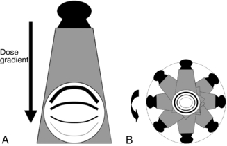
FIGURE 10-1 A, The typical dose distribution for radiographic imaging. The entrance skin dose is greater than the exit skin dose, as illustrated by the thickness of the lines, where the thicker lines denote a higher dose. B, The typical dose distribution for CT imaging showing that the dose is greater at the entrance surface of the patient (thick lines) and decreases toward the center of the patient (thin lines). From McNitt-Gray MF: Radiation dose in CT, Radiographics 22:1541-1553, 2002. Reproduced by permission of Radiological Society of North American and the author.

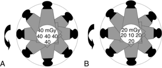
In CT, the exposure pattern is somewhat different than that of radiography because of the geometric aspects of the beam and the scanning procedure. In general, the beam is well collimated to describe a fan-shaped beam that rotates around the patient at least for 360 degrees. The x-ray tube is not fixed as in radiography but assumes several positions during one complete revolution around the patient. In modern multislice CT scanners, the fan-shaped beam has now become a cone-shaped beam (see Chapter 12). The dose distribution pattern is more uniform in CT (Fig. 10-1, B) compared with radiography because the x-ray beam is rotating 360 degrees around the patient’s body. Typical dose values for a 16-centimeter (cm) diameter head phantom and a 32-cm diameter body phantom are given in Figure 10-2, A and B, respectively.

FIGURE 10-2 Typical dose values for a 16-cm diameter head phantom (A) and a 32-cm diameter body phantom (B). From McNitt-Gray MF: Radiation dose in CT, Radiographics 22:1541-1553, 2002. Reproduced by permission of Radiological Society of North America and the author.

CT SCANNER X-RAY BEAM GEOMETRY

The term beam geometry refers to the size and shape of the x-ray beam emanating from the x-ray tube and passing through the patient to strike a set of detectors that collects radiation attenuation data. The beam geometry and scanning process of CT imaging are shown in Figure 10-3, in which a fan-shaped x-ray beam and an array of detectors rotate 360 degrees around the patient to collect attenuation data. The table moves during the scanning process, and the x-ray tube traces a spiral or helical beam path around the patient.

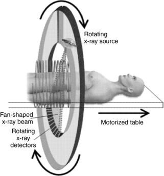
FIGURE 10-3 The scanning principles of CT imaging in which the x-ray beam and detectors rotate 360 degrees around the patient to collect attenuation data used to build up the image. In this diagram, a fan-shaped beam is used and the table moves during data acquisition to trace a spiral or helical beam path around the patient. This process is referred to as spiral or helical CT scanning. From Brenner D: Radiation risks in diagnostic radiology. In Radiological Society of North America: Categorical course in diagnostic radiology physics: from invisible to visible—the science and practice of x-ray imaging and radiation dose optimization, pp 41-50, 2006, Radiological Society of North America. Reproduced by permission of Radiological Society of North America and the author.

Figure 10-4, A, shows the same fan-shaped x-ray beam viewed from the side with the thickness exaggerated for clarity. If the longitudinal (cranial-caudal) axis of the patient is defined as the z-axis, then in theory the intensity of the radiation beam along that axis can be graphed. Ideally the radiation intensity measured along the z-axis would have equal intensity everywhere inside the beam and would have no intensity on either side. Figure 10-4, B, shows this ideal rectangular intensity profile of the radiation beam. In reality, the radiation intensity measured along the z-axis has smoother edges and appears as a bell-shaped curve. The dose distribution is almost always wider than the nominal slice width (SW).

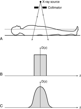
FIGURE 10-4 A, The width of the x-ray beam is viewed from the side. The collimator near the x-ray source (the width is exaggerated for clarity) determines the beam width. B, An ideal dose distribution along the z axis is shown. It has a flat top and steep sides and is the same width as the x-ray beam. C, A more realistic bell-shaped dose distribution curve is typical of most CT scanners.

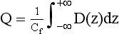
The dose distribution is given by the function D(z), which describes an arbitrarily shaped dose intensity along the patient axis. In general, the shape of D(z) varies among CT scanners. D(z) is extremely important to dose in CT because it is this dose distribution that is being measured. The instrumentation and methods used to measure patient dose from a CT scanner is referred to as CT dosimetry, and it is uniquely different compared with the dosimetry of projection radiographic imaging.

CT DOSIMETRY CONCEPTS

CT dosimetry is an important concept for CT technologists for several reasons. First, technologists can compare their hospital CT doses with the national average to find out whether their radiation protection efforts are comparable to those of others. Second, technologists can participate effectively in informing both the public and other hospital personnel (physicians and nurses, for example) about the dose in CT. Third, and perhaps more important, CT technologists can assist the medical physicist with not only performing the actual dose measurements (this has been identified as one of the duties of a certified medical physicist by the American College of Radiology) but also being a more integral part of CT acceptance testing and continuing quality control procedures. Finally, a knowledge of CT dosimetry will assist the technologist in conducting dose measurements in cases where there is no medical physicist to perform this task.

It is not within the scope of this text to describe how to conduct the actual dose measurements and how to estimate the radiation doses to patients because these are topics within the domain of medical physicists. It is important, however, to highlight several important and essential concepts, including types of dosimeters used to measure CT doses, CT dosimetry phantoms, and dose descriptors specific to CT.

Types of Dosimeters

In the past, several types of dosimeters were used to measure the dose in CT. These include film dosimeters, thermoluminescent dosimeters (TLDs), and specially designed ionization chambers. In 1981, the Bureau of Radiological Health (BRH), now the Center for Devices and Radiological Health (CDRH), introduced what could be noted as a significant step toward CT dose measurement. The method suggested by the CDRH uses a pencil ionization chamber. Recently, solid-state metal oxide semiconductor field effect transistors (MOSFET) are being used in CT dosimetry studies because they are more sensitive than TLDs and they provide an instant read out and can be reused immediately. For further details, the interested reader may refer to one such study by Mukundan et al (2007) that used MOSFET dosimetry to assess the dose to the orbits in pediatric CT imaging, for further details. In addition, those interested in the use of the TLD in CT dosimetry may refer to a report by Moore et al (2006).

Although many dose measurement methods are available, only the pencil ionization chamber method, or what the CDRH referred to as the CT dose index (CTDI) method, is described in this chapter. The ionization chamber method is the easiest and probably the most accurate, and it is used almost exclusively to report dose.

Ionization Chamber: An ionization chamber is an instrument used to accurately quantify radiation exposure. The ionization chamber shown in Figure 10-5 consists of a small air-filled container with thin walls that allow radiation to pass through easily. As the high-energy photons (x-rays) collide with air molecules enclosed within the ionization chamber, some of the molecules are “ionized” (i.e., one or more electrons are knocked from some molecules). These free electrons can be collected on a conducting wire or plate and measured as electric charge. The amount of collected charge is proportional to the amount of ionization, which is proportional to the amount of radiation that passes through the chamber. The charge is removed from the ionization chamber and measured with a very sensitive instrument known as an electrometer. The total electric charge generated by an x-ray beam is represented by Q and measured in coulombs (one coulomb = 1.6 × 10¹⁹ electrons).

FIGURE 10-5 An ionization chamber effectively performs the integral in equation 10-2 by intercepting the radiation beam and sensing the dose from all parts of the dose distribution curve. The charge emitted from the chamber is proportional to the area-under-the-dose-distribution curve.

Phantoms for CT Dose Measurement

To standardize the measurement of the dose and provide a clinically realistic geometry, the BRH researchers suggested that the ionization chamber be placed in one of two cylindrical phantoms during the radiation measurement. The smaller phantom simulates a patient’s head and the larger phantom simulates a “body” or torso (Fig. 10-6). Both phantoms are 15 cm in length. The diameter of the “head” phantom is 16 cm, and the diameter of the “body” phantom is 32 cm. Both phantoms are solid acrylic with holes drilled through the phantom at specified locations to accommodate the pencil ionization chamber (Fig. 10-7). Acrylic plugs are placed in the holes unoccupied by the ionization chamber. Figure 10-8 shows a pencil ionization chamber about to be inserted into a CT scanner dosimetry phantom. The holes that are not being used for the ionization chamber are filled with acrylic plugs. Careful examination of the plug reveals a small hole that can be seen through its diameter. This hole is centered end to end in the plug and is visible in the CT image of the dosimetry phantom if the x-ray beam is centered on the phantom and passes through the hole. The appearance of the hole in the image verifies that the x-ray beam is striking the center of the phantom.

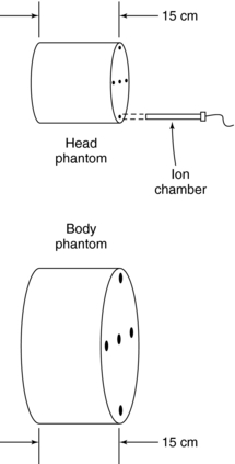
FIGURE 10-6 The “head” and “body” CT scanner dosimetry phantoms are solid acrylic with holes placed strategically to receive a pencil ionization chamber. Although the phantoms differ in diameter, they are both 15 cm long.

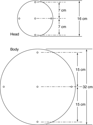
FIGURE 10-7 A view of the face of a “head” phantom (top) and a “body” phantom (bottom). Dimensions and location of the ionization chamber holes are shown. Diameters of the holes are typically 1 cm and should be drilled to match the outer diameter of the ionization chamber.

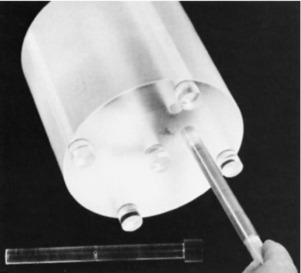
FIGURE 10-8 A pencil ionization chamber about to be inserted in a “head” CT scanner dosimetry phantom. The holes that are not being used for the ionization chamber are filled with acrylic plugs (bottom). The appearance of the hole in the image verifies that the x-ray beam is striking the center of the phantom.

The procedure for measurement is to place the ionization chamber in one of the phantom holes, take a scan, and record the amount of charge emitted from the chamber. Then the chamber is moved to the next hole, the plug is placed in the original chamber hole, and the procedure is repeated. Moving the chamber to another hole (e.g., from the anterior to the posterior) allows the dose to be determined at a variety of locations within the phantom. Generally, the dose varies among locations, even when the same technique is used. For example, the dose at the anterior location of the phantom differs from the dose at the posterior location, which differs from the dose on the patient’s right side, and so on. It is usually prudent to measure the dose at several locations for a given technique.

CT Dose Descriptors

The earlier dose studies reported CT doses by using various terms to describe the absorbed dose in a CT examination. These included single-scan peak dose, multiple-scan peak dose, dose profile, and others such as multiple-scan average dose (MSAD). These results led the CDRH to introduce and recommend the use of CTDI and MSAD in the Federal Performance Standard as the dose descriptors specific to CT. For example, because the early CT examinations consist of a series of “stop-and-go” scans (slices), the MSAD was the dose descriptor for use in a clinical situation at that time. The MSAD concept will be highlighted for historical reasons only.

Additionally, another dose descriptor, the dose length product (DLP) has been identified and used in some studies; it is available for CT scanners and is linked to the CTDI (McNitt-Gray, 2002).

Multiple-Scan Average Dose: The MSAD was the first CT dose descriptor to be identified (McNitt-Gray, 2002). To use the MSAD, a series of CT scans is performed on a patient (Fig. 10-9). Between each scan, the patient is moved a bed index (BI) distance. Each slice delivers the characteristic bell-shaped dose represented by the curves at the top of Figure 10-9. If the doses from all scans are summed, the resulting total patient dose resembles the oscillating curve at the bottom of Figure 10-9. In the regions where the bell curves overlap, the resultant dose is higher than that from just one scan. If the total dose distribution curve is known (bottom curve), the MSAD (dotted straight line) can be calculated by mathematically sampling the peaks and valleys of the multiple scan dose curve. This can be written as follows:

(10-1)

where SW is slice width in millimeters and BI is bed index or slice spacing.

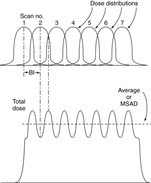
FIGURE 10-9 A series of seven scans spaced (bed indexing) apart along the z-axis disburses seven bell-shaped dose distribution curves (top). When the doses from this series are summed, the resultant total dose appears as the bottom curve. The total dose curve has peaks where the bell-shaped curves overlap. The dotted line through the total dose curve is the multiple scan average dose.

CT Dose Index: The CTDI was the next CT dose descriptor after the MSAD. It was developed by the U.S. Food and Drug Administration (FDA) and was therefore labeled CTDI_FDA (Boone, 2007). CTDI_FDA has evolved to its present form with several notable changes. These are highlighted in this subsection of the chapter.

The CTDI_FDA is defined as follows:

(10-2)

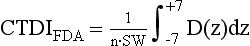
where n is the number of distinct planes of data collected during one revolution, SW is the nominal slice width in millimeters), D(z) is the dose distribution, and z is the dimension along the patient’s axis. For axial (nonspiral/helical) CT scanners and spiral/helical CT scanners with a single row of detectors, n = 1. For multislice CT scanners, n is the number of active detector rows (n = 16) during the scan.

The CTDI_FDA represents the mean absorbed dose in the scanned object volume and therefore the unit of the CTDI is the Gy with relevant submultiples such as the centigray (cGy) and the mGy.

This equation is not as complicated as it appears. The integral sign (∫) merely instructs the user to determine the area under a single curve D(z). Figure 10-10 demonstrates the value of this integral by shading the area under a typical dose distribution curve. If this area is divided by the number of slices times the slice width {(n)(SW)}, the result is the CTDI_FDA.

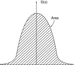
FIGURE 10-10 The integral in equation 10-2 is numerically equal to the area (shaded region) of the dose distribution curve.

This definition, which was accepted by the International Electrotechnical Commission (IEC) (IEC, 2001), is good for essentially all shapes of dose distribution curves D(z) that are emitted by CT scanners. Note that increasing the area under the curve can increase the CTDI_FDA. The area can be increased by either increasing the intensity of radiation, which raises the height of the curve, or by widening the curve, usually by opening the x-ray collimators near the x-ray tube. Either case increases the CTDI_FDA and ultimately increases the radiation dose to the patient.

For axial CT scanners, as the slice spacing increases, there is a greater likelihood that relevant tissue will be “missed” (it falls between the slices) in the scan sequence, thus limiting the amount that the BI can be increased. Conversely, when the BI is made smaller, the slices become closer together, more overlap of adjacent dose distributions occurs, and the average dose increases. When the SW equals the BI, the MSAD is numerically equal to the CTDI_FDA.

The CTDI_FDA has evolved from its initial stage of measurement for 14 contiguous slices where the integration would be from −7 to +7. The fixed length of the pencil ionization chamber “meant that only 14 sections of 7-mm thickness could be measured with that chamber alone. To measure CTDI_FDA for thinner sections, sometimes lead sleeves were used to cover the part of the chamber that exceeded 14 section widths” (McNitt-Gray, 2002).

This shortcoming was solved by introducing another dose index, the CTDI₁₀₀, which “relaxed the constraint on 14 sections and allowed calculation of the index for 100 mm along the length of the entire pencil ionization chamber, regardless of the nominal slice width being used” (McNitt-Gray, 2002). The index is given by the equation

(10-3)

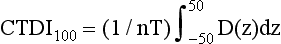
where nT is the nominal collimated slice thickness.

The next major change in the CT dose descriptor is the introduction of the weighted CTDI (CTDI_W) to account for the average dose in the x-y axis of the patient instead of the z-axis. This can be done using a phantom where the pencil ionization chamber is positioned in the center (CTDI_center) and at the periphery (CTDI_periphery) of the phantom (see Fig. 10-7). In this case the following algebraic expression can be used to calculate the CTDI_W as provided by McNitt-Gray (2002):

(10-4)

Several examples of the CTDI_W for head and body dose phantoms at 120 kilovolts (kV) for five CT scanners are given in a report by Huda and Vance (2007). They state that for the following scanners; LightSpeed Plus (GE Healthcare), Mx8000 IDT (Philips Medical Systems), Sensation 16 (Siemens Medical Solutions), 7000 TS (Shimadzu Corporation), and the Aquilion Multi (Toshiba Medical Systems), the CTDI_W (mGy/milliampere [mA]) for the head were 0.180, 0.130, 0.190, 0.180, and 0.190 respectively. For the body, the CTDI_W were 0.094, 0.066, 0.069, 0.103, and 0.105, respectively.

To consider the dose in the z-axis, yet another dose descriptor was developed. This is the CTDI_volume, which can be calculated with the following relationship for spiral//helical CT imaging:

(10-5)

It is important to note that the term pitch has been defined by the IEC as a ratio of the distance the table travels per revolution (in millimeters) to the total nominal beam collimation (in millimeters). For a pitch of 1, the CTDI_volume is equal to the CTDI_W; for a pitch of 1.5, the CTDI_volume is equal to CTDI_W/1.5.

Dose Length Product: As mentioned earlier, the DLP is yet another dose descriptor used in CT dose studies and reported in the literature and on CT scanners. Although the CTDI_volume provides a measurement of the exposure per slice of tissue, the DLP provides a measurement of the total amount of exposure for a series of scans. The DLP can be calculated if the length of the irradiated volume (scan length) and the CTDI_volume are known by using the following relationship:

(10-6)

It is important to note that, although the CTDI_volume is not dependent on the scan length, the DLP is directionally proportional to the scan length.

In summary, McNitt-Gray (2002) informs the radiologic community that “these CTDI descriptors are obviously meant to serve as an index of radiation dose due to CT scanning and are not meant to serve as an accurate estimate of the radiation dose incurred by an individual patient. Although the phantom measurements are meant to be reflective of an attenuation environment somewhat similar to a patient, the homogeneous polymethyl methacrylate phantom does not simulate the different tissue types and heterogeneities of a real patient.”

Measuring the CT Dose Index: It is not within the scope of this book to describe the details of how to measure the CTDI because this is a task for the medical physicist. However, the following steps are noteworthy, using the phantoms and pencil ionization chamber described earlier:

1. The pencil ionization chamber is placed into one of the holes in the phantom, perpendicular to the fan of the radiation beam (i.e., the chamber is placed parallel to the longitudinal axis of the patient) (see Fig. 10-5), and the other holes are plugged with acrylic plugs.

2. An exposure is made for a single scan, and the chamber measures the exposure (not dose). The chamber intercepts the entire narrow width of the x-ray beam. The x-ray beam must be positioned in the center of the chamber.

3. The chamber converts the x-rays into charge. This charge represents the integral in Equation 10-2.

4. The ionization chamber receives radiation from all parts of the dose distribution D(z) because of its length. The total charge from the ionization chamber is proportional to the integral in the CTDI definition. Mathematically, this is expressed as follows:

(10-7)

where Q is the total charge collected during a single scan and C_f is the calibration factor of the ionization chamber. Because the ionization chamber measures exposure and not the dose, a conversion factor (the f factor) must be included in C_f, which converts exposure (in Roentgens) to dose (cGy; recall that 1 cGy = 1 rad). The value of the f factor at CT scanner x-ray energies is approximately 0.94 cGy/Roentgen.

An interesting point to note about the CTDI is that the integration range is restricted to single-slice CT scanners collimated to beam widths of 10 mm and less (Boone, 2007) and to 100 mm for the CTDI₁₀₀. As pointed out by Cody and McNitt-Gray (2006), “with the advent of multidetectors scanners with beam widths from 25 to 40 mm (and a prototype that has a nominal collimated beam width of 128 mm (Mori et al, 2006), the 100 mm pencil chamber will not be able to capture all of the primary and scatter radiation in the CTDI phantoms. In addition, CTDI is measured in a single transverse scan so that the pencil chamber can integrate the radiation dose profile, assuming a contiguous transverse scanning protocol; approximations are made to calculate dose when helical scanning is performed.…therefore, methods are being developed to measure radiation dose better for multidetector CT (and also for cone beam CT) as well as to measure estimated actual radiation does to patients.” For example, the nominal beam width for the 256-slice CT scanner is 128 mm; therefore, the integration range has increased to 300 mm for an accurate measurement of the dose from this CT scanner (Mori et al, 2006). These investigators have developed what they call the dose profile integral (DPI). In addition, in a letter to the editor of Medical Physics, Dixon (2006) proposes that a Farmer ion chamber be used to measure the dose with a phantom “using the exact protocol that would be used for patients, instead of a single transverse scan, removing the need to make approximations or corrections for helical scanning” (Cody and McNitt, 2006). Other investigators have used MOSFET technology as well to assess dose in CT (Dixon, 2003; Muhundan et al, 2007.

These measurement and dose estimation methods are not described further in this text; however, the interested reader should refer to the reports by Dixon (2003, 2006).

FACTORS AFFECTING DOSE IN CT

Several factors affect the dose in CT. These fall into two categories, namely, those that have a direct effect on the dose and those that have an indirect effect on the dose (Cody and McNitt-Gray, 2006; Kalra et al, 2004a; McNitt-Gray, 2002). Although the direct factors are those factors that increase or decrease the dose to the patient and are under the direct control of the technologist, the indirect factors are those that “have a direct influence on image quality, but no direct effect on radiation dose; for example, the reconstruction filter” (McNitt, 2002). It is beyond the scope of this chapter to describe all of these factors; however, only the factors that have a direct effect on the dose to the patient, and which the technologist has some degree of control, are reviewed. These include the exposure technique factors, x-ray beam collimation, pitch, patient centering, number of detectors, and overranging, also referred to as z-overscanning.

Exposure Technique Factors

Exposure technique factors are characterized by the tube potential defined by the kilovoltage; tube current, defined by the milliamperage; and the exposure time in seconds. The product of the milliamperage and the exposure time is the milliamperage-seconds (mAs). The technologist can select these factors manually or they can be selected by using AEC. AEC uses a technique known as automatic tube current modulation, which is described later in the chapter.

Constant Milliamperage-Seconds: The term constant mAs refers to the selection of milliamperage and time (in seconds) separately or mAs on some scanners before the scan begins, keeping all other technical factors constant. The mAs determines the quantity of photons (dose) incident on the patient for the duration of the exposure. The dose is directly proportional to the mAs, and therefore if the mAs is doubled, the dose will be doubled. The results of different amounts of mAs on the dose (mGy and mGy/mAs) using a phantom and a 64-slice CT scanner are provided in Table 10-1. It is clearly apparent that as the mAs increases, the dose increases proportionally. For example, the CTDI_w (mGy) for a 32-cm diameter body phantom using 110 mAs and 220 mAs is 7.4 and 15 mGy, respectively, when all other technical scanning factors remain constant (Cody and McNitt-Gray, 2006).

TABLE 10-1

Changes in CTDI_w in a 32-cm Diameter Body Phantom as a Function of Tube Current-Time Product for Both Constant Rotation Time Settings and Constant Current Settings

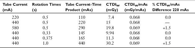
Note: All other factors were held constant at 120 kVp with 20 channels and 1.2-mm channel width (20 × 1.2 mm).

From Cody, McNitt-Gray: CT image quality and patient radiation dose: definitions, methods, and trade-offs. In Radiological Society of North America: Categorical course in diagnostic radiology physics: from invisible to visible—the science and practice of x-ray imaging and radiation dose optimization, Chicago, 2006, Radiological Society of North Ameria. Reproduced by permission of Radiological Society of North America and the authors.

Effective Milliamperage-Seconds: The effective mAs is a term used for multislice CT scanners that denotes the mAs per slice. This is given by the following relationship:

(10-8)

This expression simply implies that, to keep the effective mAs constant, as the pitch increases, the true mAs must be increased as well (Cody and McNitt-Gray, 2006). For example, increasing the pitch from, say, 1 to 2, increases the mAs per rotation from 100 to 200 while the relative CTDI_vol remains the same (Lewis, 2005).

Peak Kilovoltage: The peak kilovoltage (kVp) determines the penetrating power of the photons coming from the x-ray tube. Higher kVp means that the photons have higher energies and can penetrate thicker objects compared with lower kVp x-ray beams. In CT generally, for adult imaging, high kVp techniques are used, such as 120 kVp, for example. The radiation dose is proportional to the square of the kVp (Bushberg et al, 2004). This means that the quantity of photons increases by the square of the kVp. A 72-kVp technique will have fewer photons than a kVp of 82, all factors held constant.

The results of different amounts of kVp on the dose (mGy and mGy/mAs) with a 64-slice spiral/helical CT scanner are provided in Table 10-2. It is clearly apparent that as the kVp increases, the dose increases. For example, the CTDI_w (mGy) for a 32-cm diameter body phantom using an 80 kV and a 140 kVp beam is 5.2 and 24.9 mGy, respectively, when all other technical scanning factors remain constant (Cody and McNitt-Gray, 2006).

TABLE 10-2

Changes in CTDI_w in a 32-cm Diameter Body Phantom as a Function of Tube Potential (kV)

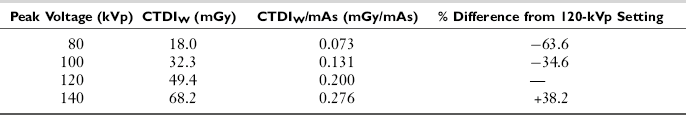
Note: All other factors were held constant at a 0.75-second rotation time, 330 mA, collimation of 12 channels with 1.5-mm channel width (12 × 1.5 mm), and head bowtie filtration.

From Cody, McNitt-Gray: CT image quality and patient radiation dose: definitions, methods, and trade-offs. In Radiological Society of North America: Categorical course in diagnostic radiology physics: from invisible to visible—the science and practice of x-ray imaging and radiation dose optimization, Chicago, 2006, Radiological Society of North America. Reproduced by permission of Radiological Society of North America and the authors.

Collimation (Z-Axis Geometric Efficiency)

In CT, the collimation is used to define the beam width for the examination. Collimation schemes are different between single-slice (single detector row along the z-axis) and multislice (multidetector rows along the z-axis) CT scanners. The collimation reflects the efficient use of the x-ray beam at the detector, as shown in Figure 10-11. The shaded portion represents the penumbra that is caused by the finite size of the x-ray tube focal spot. It is clearly apparent that on a single-slice CT scanner the entire beam width plus the penumbra fall on the detectors. The penumbra, however, is not used to produce the image, but it does affect the patient dose.

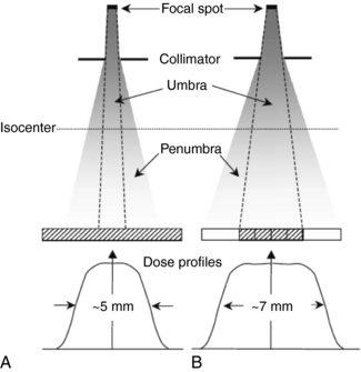
FIGURE 10-11 The implications of focal spot penumbra on dose. In A the geometry of a single-slice scanner collimated to a nominal slice width of 4 mm is illustrated. The umbra and all the penumbra contribute to image formation, resulting in a dose profile of 5 mm that, when corrected to the isocenter, closely corresponds to the nominal slice width of 4 mm. In B the geometry for a multislice scanner collimated to a nominal 4 × 1 mm beam width may be compared. The collimators must be opened to ensure that each of the four 1-mm wide detector rows receives similar umbral radiation. The penumbral radiation is not used in the image reconstruction, and the resulting dose profile is approximately 7 mm in width. From Heggie JCP et al: Importance of optimization of multi-slice computed tomography scan protocols, Aust Radiol 50:278-285, 2006. Reproduced by permission of Blackwell Publications, Oxford, England.

On multislice CT scanners, the beam width, including the penumbra, would fall on a finite set of detectors depending on the scanner, but the penumbra would not be used to produce the image (because the intensity of the beam at the penumbra regions is less than the intensity at the center of the beam). To address this problem, the beam width (collimation) is increased so that the penumbra extends beyond the active detectors that will receive the central beam intensity (Lewis, 2005). The ratio of the area under the z-axis dose profile falling on the active detectors to the area under the total z-axis dose profile is referred to as the z-axis geometric efficiency (IEC, 2001).

Cody and McNitt-Gray (2006) have shown that for a 32-cm diameter phantom, as beam widths increase from 18.0 mm, 19.2 mm, 24.0 mm, and 28.8 mm, the CTDI_w (mGy) changes from 15.7 mGy, 16.8 mGy, 15.0 mGy, and 13.9 mGy, respectively (all other technical factors held constant). Additionally, Lewis (2005) indicates that “scanners that acquire a greater number of simultaneous slices have an advantage in terms of z-axis geometric efficiency. This is because for narrow slice widths a wider total collimation can be used.…On multislice scanners z-axis geometric efficiencies are generally in the range of 80-98% for collimators of 10mm and above, and about 55-75% for collimators of around 5mm. For collimators around 1-2mm z-axis geometric efficiencies are as low as 25% on some systems, although in dual slice mode, they can be much higher. Therefore the reduced geometric efficiency of multislice scanners, for wider collimators most commonly used, leads to dose increases around 10% when compared to single slice systems. However very narrow collimations can result in a tripling, or more, in dose.”

Pitch

The term pitch is one common to spiral/helical CT scanners, sometimes called spiral pitch or helical pitch depending on the manufacturer of the scanner. As defined by the IEC, pitch is a ratio of the distance the table travels per rotation to the total collimated x-ray beam width. The relationship between the absorbed dose and pitch is as follows:

(10-9)

Therefore if the pitch increases by 2, the dose will be reduced to one half. It is important, however, to note that this relationship only holds true when the pitch changes and all other factors remain constant. For constant mAs (100 mAs per rotation), if the pitch changes from 1 to 2, the relative CTDI_vol decreases from 1.0 to 0.5mGy (Lewis, 2005).

Number of Detectors

In a study comparing the dose from multislice CT scanners, Moore et al (2006) demonstrated that the measured radiation dose is inversely proportional to the number of detector rows. They showed that there is a trend that as the number of detector rows increases from 4, 8, to 16 detector rows, the dose decreases with both standard and near identical technique (Moore et al, 2006).

Overranging (Z-Overscanning)

In spiral/helical CT scanning, it is important to realize that to image the planned length of tissue required for the examination and that is of interest to the radiologist, additional rotations before and after the planned length are essential for the image reconstruction process. This is referred to as overranging or z-overscanning (Van der Molen and Gelijns, 2007; Tzedakis et al, 2007), of which the components and definitions developed by Van der Molen and Gelijns (2007) are clearly illustrated in Figure 10-12. It is clear that there are two definitions of overranging:

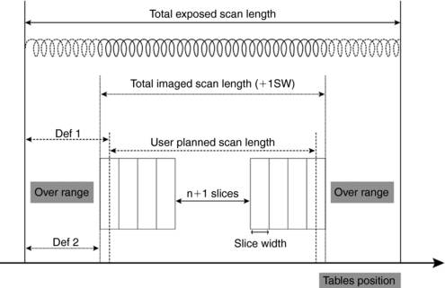
FIGURE 10-12 Simplified depiction of overranging components and definitions at helical CT scanning. To the planned scan length, one section width (SW) is automatically added so imaged scan length is slightly longer. Extra rotations needed for image reconstruction are added to imaged length, resulting in longer exposed scan length. Definitions of overranging vary; either the difference between planned and exposed scan length (Def 1) or the difference between imaged and exposed scan length (Def 2) is used. From Van der Molen AJ, Geleijns J: Overranging in multisection CT: quantification and relative contribution to dose—comparison of four 16-section CT scanners, Radiology 242:208-216, 2007. Reproduced by permission of Radiological Society of North America and the authors.

1. Definition 1: This refers to the difference between the planned and exposed scan length.

2. Definition 2: This refers to the difference between the imaged and the exposed scan length.

Overranging increases the dose to the patient, which is validated in studies conducted by Tzedakis et al (2007) on pediatric patients and by Van der Molen and Gelijns (2007). For example, Tzedakis et al (2007) concluded that “in all cases normalized effective dose values were found to increase with increasing z-overscanning. The percentage differences in normalized data between axial and helical scans may reach 43%, 70%, 36%, and 26% for head-neck, chest, abdomen-pelvis, and trunk studies, respectively.” Van der Molen and Gelijns (2007), for example, concluded that “overranging is reconstruction algorithm specific, and its length generally increases with collimation and pitch, while the effect of section width is variable. Overranging may lead to substantial but unnoticed exposure to radiosensitive organs.”

Patient Centering

Another factor affecting the dose to the patient that is under the control of the technologist is that of patient centering. The patient must be centered in the gantry isocenter for accurate imaging of the anatomy. Inaccurate patient centering (miscentering) as shown in Figure 10-13 degrades the image quality and increases the dose to the patient, especially with the use of AEC in CT (Li et al, 2007; Toth et al, 2007). Additionally, the use of bowtie filters in CT scanners is intended to serve basically two purposes: to shape the beam intensity within the scan field-of-view (SFOV) and to produce a more uniform beam at the detectors (Chapter 5). The x-ray beam is filtered; therefore, the bowtie filter actually plays a small role in reducing the dose to the patient because the low energy photons are removed and thus the beam becomes harder, that is, the mean energy of the beam increases. Improper centering of the patient in the gantry isocenter as shown in Figure 10-13 can lead to an increase in surface dose as well as the peripheral dose to the patient (Li et al, 2007; Toth et al, 2007).

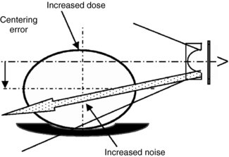
FIGURE 10-13 A patient who is miscentered in the scan field of view can be expected to have degraded bowtie filter performance with an undesired increase in both dose and noise. From Toth et al: How patient centering affects CT dose and noise, Med Phys 34:3093-3101, 2007. Reproduced by the American Association of Physicists in Medicine.

In a study on the effect of patient centering on CT dose and image noise, Toth et al (2007) showed that, for a 32-cm CTDI body phantom, a miscentering of about 3 cm and 6 cm can result in an increase in doses by 18% and 41%, respectively. Similar results were obtained by Li et al (2007). Furthermore, a miscentering in elevation by 20 to 60 mm with a mean position 23 millimeters below the isocenter can result in a dose increase of up to 140% “with a mean dose penalty of 33% assuming that the tube current is increased to compensate for the increased noise due to miscentering” (Toth et al, 2007).

These findings are positive proof that technologists should always center the patient accurately in the gantry isocenter to avoid image noise problems and reduce the dose to the patient.

Automatic Tube Current Modulation

AEC is now commonplace on CT scanners. AEC uses a technique referred to as automatic tube current modulation (ATCM) to optimize the dose to the patient while maintaining constant image quality regardless of the size of the patient in the z-axis and the attenuation changes in the x-y axis (Brisse et al, 2007; Toth et al, 2007). ATCM has been hailed as “the most important technique for maintaining constant image quality while optimizing radiation dose” (Li et al, 2007). For this reason, ATCM is described in detail in the next section of the chapter.

AUTOMATIC TUBE CURRENT MODULATION

ATCM is a technical development in CT based on the fundamental principles of AEC. AEC is not a new concept for radiologic technologists, for it is used extensively in radiography and fluoroscopy. The purpose of AEC in radiography, for example, is to provide a level of image quality (expressed as optical density for film-based radiography) in which there is consistent optical density for any examination (e.g., chest x-ray) regardless of the thickness (small, medium, and large) of the patient. This level of image quality (optical density) is controlled by varying the duration of the exposure on the basis of the size of patient being imaged. For example, although the duration of the exposure will be shorter for smaller patients, it will be longer for larger patients, and therefore images of the same body parts on these patients will all have a consistent level of optical density.

Problem with Setting Manual Milliamperage Techniques

In CT, the exposure technique factors (mAs and kVp) do not have a direct effect on the image density and contrast, respectively (as they do in film-based radiography), because CT is a digital imaging modality. The dose to the patient is directly proportional to the mA, and in the past, CT technologists selected the mA values for patients manually. Lewis (2005) explains one of the problems with setting the mA values manually. She notes “the attenuation of the x-ray beam increases with the thickness of material in its path, and for approximately every 4 cm of soft tissue, the x-ray beam intensity halves. In order to achieve the same transmitted x-ray intensity, and thereby the same level of image noise, changing from a 16 cm to a 20 cm diameter phantom requires a doubling of the mA. Changing from a 32 cm to a 48 cm phantom, the mA should in theory, be increased by a factor of 16. Systems which automatically adapt the overall tube current based on actual patient attenuation remove the guesswork from selecting the appropriate mA setting” (Lewis, 2005).

Definition of Automatic Tube Current Modulation

In CT, ATCM refers to the automatic control of the mA in two directions of the patient (the x-y axis and the z-axis) during data acquisition (scanning process) by use of specific technical procedures that take into consideration not only the patient size but also the attenuation differences of the various tissues. The overall goal of ATCM is to provide consistent image quality despite the size of the patient and the tissue attenuation differences and to control the dose to the patient (Brisse et al, 2007; Kalra et al, 2004b; Li et al, 2007; McCollough et al, 2006; Toth et al, 2007) compared with manual mA selection techniques. Although the automatic control of the tube current (mA) in the x-y axis (in-plane) is referred to as angular modulation, changing the tube current automatically in the z-axis (through-plane) is referred to as z-axis modulation or longitudinal modulation. When used together, that is, angular-longitudinal tube current modulation, AEC is the result (Goodman and Brink, 2006).

The use of angular-longitudinal modulation can reduce the dose by as much as 52% compared with use of only the angular modulation technique (Goodman and Brink, 2006).

Historical Background

ATCM techniques can be traced back to 1981, when Haaga et al (1981) suggested its use as a dose reduction strategy in CT while not compromising the needed image quality to make a diagnosis. This was followed by efforts of several others, such as General Electric (GE) Medical Systems in 1994 and researchers such as Kalender, who in 1999 published two reports describing dose reductions as much as 40% with ATCM techniques (McCollough et al, 2006). Later in 2001, a number of CT manufacturers such as GE Healthcare, Philips, Siemens, and Toshiba introduced ATCM techniques referred to by several names. For example, angular modulation systems are referred to as Smart Scan (GE Healthcare), DOM-Dose Modulation (Philips), and Care Dose (Siemens). In addition, different names are used for both angular-longitudinal modulation systems, such as for example; Smart mA (GE Healthcare), Z-DOM (Philips), CareDose 4D (Siemens), and Sure Exposure (Toshiba).

Basic Principles of Operation

In CT AEC, the tube current (mA) is adjusted in real time during the scanning of a patient on the basis of differences in radiation attenuation in the transverse or x-y direction (in-plane) and the z-axis or longitudinal direction (through-plane) during the rotation of the tube and detectors. In addition, these tube current modulation techniques require some knowledge of the attenuation characteristics of the patient, and second, the operator must first set up the defined level of image quality (image noise target value) needed for the examination (Cody and McNitt-Gray, 2006; Lewis, 2005; McCollough et al, 2006). Each of these will be described briefly.

Longitudinal (Z-Axis) Tube Current Modulation: Longitudinal (z-axis) tube current modulation (z-axis TCM) is based on differences in attenuation among body parts. For example, thicker body parts such as the abdomen and pelvis will attenuate the radiation more than thinner body parts, such as the head, neck, and chest regions. The technique of z-axis TCM is designed (using a specific computer algorithm) to change the mA automatically as the patient is scanned from, say, head to toe (along the z-axis) while maintaining a constant (uniform) noise level (image noise target values) for different thicknesses of body parts examined. This is clearly shown in Figure 10-14.

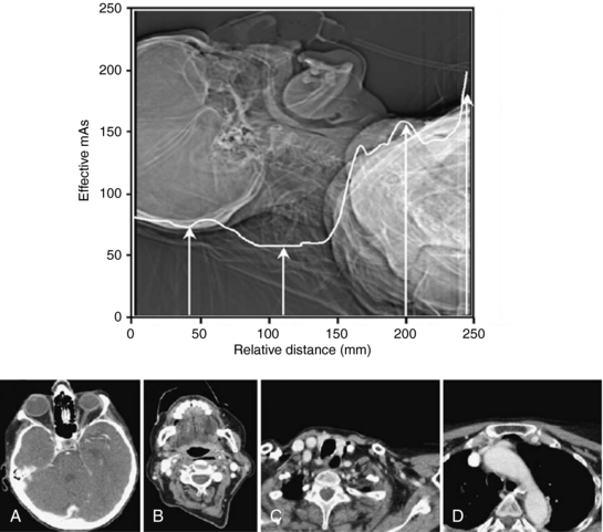
FIGURE 10-14 The z-axis tube current modulation during CT of the neck. On the basis of the attenuation measurements made during the acquisition of the scan projection radiograph, the scanner software adjusts the effective mAs on the fly during the acquisition of the axial images. Axial images shown through orbits (A), midcervical vertebrae (B), the apex of the lung (C), and the aortic arch (D) require 75, 58, 160, and 200 mAs respectively, at 120 kVp. From Heggie JCP et al: Importance of optimization of multi-slice computed tomography scan protocols, Aust Radiol 50:278-285, 2006. Reproduced by permission of Blackwell Publications, Oxford, England.

Angular (X-Y Axis) Tube Current Modulation: Angular (x-y axis) tube current modulation (x-y axis TCM) is based on the fact that the radiation attenuation varies from the anteroposterior (AP) projection (low attenuation) to the lateral projection (high attenuation) as the tube rotates around (gantry rotation) the patient. Although the high attenuation projections will require higher mA values, the low attenuation projections will require lower mA values, as illustrated in Figure 10-15. The x-y axis TCM algorithm ensures that a constant (uniform) noise level is maintained during the scanning process.

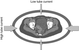
FIGURE 10-15 Angular modulation with CARE Dose (Siemens Medical Solutions) ATCM technique. On-line modulation of tube current is performed at different projections in the x-y plane within each 360-degree x-ray tube rotation. Thin arrows indicate reduction of tube current relative to higher tube current (thick arrows). From Kalra M et al: Techniques and applications of automatic tube current modulation for CT, Radiology 233:649-657, 2004. Reproduced by permission of the Radiological Society of North America and the authors.

Angular-Longitudinal Tube Current Modulation: Figure 10-16 illustrates a method where both x-y axis and z-axis modulation can be used together to therefore provide the “most comprehensive approach to CT dose reduction because the x-ray dose is adjusted according to the patient-specific attenuation in all three planes” (McCollough et al, 2006).

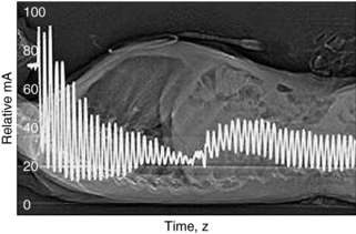
FIGURE 10-16 Graph of tube current (mA) superimposed on a CT projection radiograph shows the variation in tube current as a function of time (and, hence, table position along the z-axis) at spiral CT in a 6-year-old child. An adult scanning protocol and an AEC system (CareDose 4D, Siemens Medical Solutions) were used with a reference effective tube current-time product of 165 mAs. The mean effective tube current-time product for actual scanning was 38 mAs (effective tube current-time product = tube current-time product/pitch). From McCollough C et al: CT dose reduction and dose management tools: overview of available options, Radiographics 26:503-512, 2006. Reproduced by permission of the Radiological Society of North America and the authors.

Approaches to Obtaining Attenuation Characteristics of the Patient: The attenuation characteristics of the patient are one of the first pieces of information that is required to use of AEC systems in CT imaging (that is, vary the mA during the scanning process and keep the image noise constant regardless of the gantry rotation and the z-axis position). Such information is currently obtained by two different schemes. Although the first approach uses a CT scanned projection radiograph (SPR), the typical “scout view” (also referred to as ScoutView, Topogram, or the Scanogram depending on the CT vendor), the second approach makes use of “on-line” data “from the preceding 180° of rotation to modulate the mA” (Lewis, 2005).

Defined Level of Image Quality in CT Automatic Exposure Control: The second requirement when AEC is used in CT imaging is that operators must set up the defined level of image quality on their respective CT scanners. The approaches from four CT vendors include a noise index (GE Healthcare), a reference image (Philips), a quality reference mAs (Siemens), and the standard deviation of CT numbers or an image quality level (Toshiba). Each of these is briefly described in Table 10-3. Essentially, the fundamental basis for these methods, as outlined in Table 10-1, rests on several important points:

TABLE 10-3

Image Quality Paradigms to Help the Computed Tomography Operator Select the Desired Level of Image Quality in Automatic Exposure Control in Computed Tomography

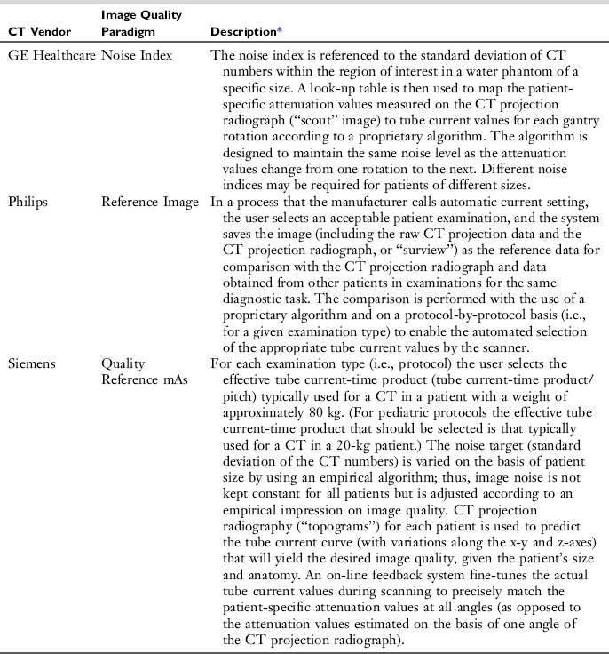
^*McCollough et al: CT dose reduction and dose management tools: overview of available options, Radiographics 26:503-512, 2006.

1. A CT projection radiograph is required from which attenuation data are obtained.

2. An image quality index is prescribed (prescription of the mA). This index related to the noise level (standard deviation of the CT numbers in a water phantom) (Lewis, 2005), or

3. A referenced image is selected (from previous examinations) that has the image quality required and the mA is adjusted to produce the same level of image quality as the referenced image when scanning other patients.

4. These methods are based on the use of proprietary algorithms.

IMAGE QUALITY AND DOSE: OPERATOR CONSIDERATIONS

It is clearly apparent from the foregoing discussion that image quality and dose are closely related. Image quality includes spatial resolution, contrast resolution, and noise. Although spatial resolution depends on geometric factors (such as focal spot size, slice thickness, and pixel size, for example), contrast resolution and noise depend on both the quality (beam energy) and quantity (number of x-ray photons) of the radiation beam. Several mathematical equations have been derived to express the relationship between dose and image quality (Bushong, 2009). For CT operators, the following mathematical expression is important:

where intensity and beam energy depend on mA and kVp, respectively, and noise depends on the number of photons detected. This expression is read as follows: dose is directly proportional to the product of mA and kVp and inversely proportional to the product of noise squared, pixel size cubed, and slice thickness.

The expression also implies the following about dose and image quality:

1. To reduce the noise in an image by a factor of 2 requires an increase in the dose by a factor of 4.

2. To improve the spatial resolution (pixel size) by a factor of 2 (keeping the noise constant) requires an increase in the dose by a factor of 8.

3. To decrease the slice thickness by a factor of 2 requires an increase in the dose by a factor of 2 (keeping the noise constant).

4. To decrease both the slice thickness and the pixel size by a factor of 2 requires an increase in the dose by a factor of 16 (2³ × 2 = 2 × 2 × 2 × 2).

5. Increasing mA and kVp increases the dose proportionally. For example, a twofold increase in mA increases the dose by a factor of 2. Additionally, doubling the dose will require an increase by the square of the kVp.

CT DOSE OPTIMIZATION

In this chapter, two points have been made clear so far. First, CT is rapidly expanding in its use in medicine. Second, a major concern that is receiving increasing attention in the literature relates to the potential for high radiation doses delivered by CT scanners and the potential biologic risks of CT scanning (Brenner and Elliston, 2004; Brenner et al, 2001). With these notions in mind, there have been increasing efforts to reduce the dose to the patient without compromising the image quality needed to make a diagnosis. One such significant approach is that of dose optimization, and to date various strategies have been devised to help CT users reduce the dose to the patient while maintaining optimal image quality (Heggie et al, 2006; Kalra et al, 2004a; Lewis, 2005; McCollough et al, 2006).

What Is Dose Optimization?

Optimization is a radiation protection principle that is intended to ensure that doses delivered to patients are kept as low as is reasonably achievable (ALARA). Essentially, the principle of optimization refers to reducing radiation dose while maintaining the required image quality needed for making a diagnosis. Dose optimization is especially important for digital imaging modalities such as computed radiography and CT, for example, where the potential for high doses exists (Brenner and Hall, 2007).

Dose Optimization Strategies

As described in this chapter, a number of factors affect the dose to the patient in CT. These include the scan parameters such as exposure technique factors (constant and effective mAs and kVp), collimation (z-axis geometric efficiency), pitch, number of detectors, overranging (z-overscanning), patient centering, and ATCM. To effectively reduce the dose and maintain the needed image quality, users must have systematic approaches or strategies to CT dose optimization.

Several authors have described various dose optimization strategies in CT, especially in multislice CT (Frush, 2004; Heggie et al, 2006; Kalra et al, 2004a; Kanal et al, 2007; Lai and Frush, 2006; Lewis, 2005; McCollough et al, 2006; Winkler, 2003; Winkler and Mather, 2005). It is not within the scope of this chapter to describe details of these strategies; however, it is noteworthy to highlight the essential guiding principles. Several strategies that emerge as common themes relate to the mAs, kVp, collimation, slice thickness, scanned volume, pitch, and the use of ATCM techniques. In CT dose optimization, Heggie et al (2006) present a summary of the main items to consider, as listed in Box 10-1.

BOX 10-1 Optimization Technique

Use sequential as opposed to helical techniques for head scans

Avoid transferring scan protocols applicable to one scanner to another without due consideration to differences in scanner filtration and geometry

Keep scanned volume to minimum and scan in one large block rather than multiple smaller blocks. However, see text for possible exceptions

Use widest x-ray beam collimation consistent with clinical requirements

Consider using a lower tube potential for CT angiography

Keep the effective mAs, which is defined as the mAs/pitch, as low as clinically indicated

Use tube current modulation technology with an appropriately selected reference effective mAs or noise index. For optimum performance of modulation technology, the SPR that is of clinical relevance must be acquired over the full length of the patient by using the same kVp that will be subsequently used for the axial image acquisition

Minimize use of multiphasic examinations

The primary parameters that have an impact of CT dose optimization.

From Heggie et al: Importance in optimization of multi-slice computed tomography scan protocols, Aust Radiol 50:278-285, 2006. Reproduced by permission Blackwell Publishing Limited, Oxford, England.

Dose optimization has received increasing attention in pediatric CT. Lai and Frush (2006) and Goodman and Brink (2006), for example, present excellent overviews on this topic, examining not only trends and patterns of CT use, radiation risks from CT, and how radiologists can manage CT dose but also focus on the technical factors for dose management such as controlling tube current and voltage, the influence of gantry cycle time, choice of pitch and detector width, and finally the use of tube current modulation techniques. For example, Lai and Frush (2006) emphasize the importance of the radiologist to ensure that all examinations ordered should be justified and that the need for communications between ordering physicians and radiologists is vital as a first step to CT dose reduction. Additionally, they point out that the CT protocols used must include various technical parameters that optimize the dose to the patient without compromising the needed image quality. In this regard, they state that increasing the detector width from 0.625 to 1.25 for a 16-slice CT scanner while holding all other factors constant will result in a reduced dose to the patient. Finally, they also advocate the use of age- or weight-adjusted CT protocols and the use of ATCM techniques. In addition, interesting study on optimizing image quality and radiation dose in CT pulmonary angiography showed that by decreasing the peak kilovoltage from 120 to 100 kVp, the dose to the patient is reduced significantly without loss of objective or subjective image quality (Heyer et al, 2007).

RADIATION PROTECTION CONSIDERATIONS

The dose optimization strategies described so far focus on methods to reduce the dose to the patient. What about the protection of personnel in CT scanning? Radiation protection of both patients and personnel in medicine is guided by two triads that are intended to ensure that medical radiation workers work within the ALARA (as low as reasonable achievable) philosophy of the ICRP. One triad deals with radiation protection actions, and the other triad addresses the radiation protection principles (Seeram, 2001).

Radiation Protection Actions

Radiation protection actions include the use of time, shielding, and distance, which are intended to protect both patients and personnel in radiology. For example, because dose is proportional to the time of exposure, to protect personnel in CT, it is essential to minimize the time spent in the CT scan room during the exposure.

Distance, on the other hand, is a major dose reduction action because the dose is inversely proportional to the square of the distance. This means that the further one is away from the radiation source, the less the dose received. In CT, because the patient is the main source of scatter, technologists should stand back as far away from the patient as possible if there is a need to be present in the scan room during scanning. This implies that the use of a power injector that can be controlled from outside the scan room is recommended. If a hand injector is used, then a long tubing should be used.

Shielding is intended to protect not only patients (gonadal, breast, eyes, and thyroid shielding) but also personnel and members of the public. Patients are often concerned about the exposure of their gonads during a CT examination. Because most of the gonadal exposure will come from internal scatter and not from the primary beam (unless the gonadal region was being examined), there is no need for this concern. Technologists, however, could place gonadal shielding on the patient because it may alleviate any fears about the risks of being exposed to radiation. Shields can also be used to protect the eyes, breast, and thyroid of patients undergoing CT examinations (Fricke et al, 2003; Kennedy et al, 2007). Although some of the shields are made of flexible, nonlead (bismuth) composition, lead may also be used (Kennedy et al, 2007) to provide significant dose reduction to these critical organs.

When personnel are expected to be present in the CT scan room during the exposure, lead aprons should be worn (for the same reason that gonadal shields are placed on patients) because of the presence of scatter (Bushong, 2009).

Because scatter radiation is present during a CT examination and strikes the walls of the CT room, should these walls be shielded to protect members of the public or other radiation workers who are present outside the room. The use of minimum shielding in the form of thick plate-glass control room viewing windows and gypsum wall board with no lead content can sometimes provide the minimum required shielding.

Radiation Protection Principles

Radiation protection principles deal with justification, optimization, and dose limitation, principles that are vital to radiation protection regulation.

Justification involves the concept of net benefit, that is, there must be a benefit associated with every exposure. This requirement is intended for referring physicians and is one effort to reduce doses to patients undergoing x-ray examinations.

Optimization is a principle that is intended to ensure that doses delivered to patients are kept as low as is reasonably achievable (ALARA), economic and social factors being taken into account. In implementing ALARA, technologists should always apply all relevant technical radiation protection practices to ensure that the dose is optimized and that image quality is not compromised, as discussed earlier in the chapter.

The concept of dose limitation is a major integral component of regulatory guidance on radiation protection. This concept addresses the dose that an individual receives annually or accumulates over a working lifetime. These doses should be within the limits established by international organizations such as the ICRP and other national bodies such as the National Council on Radiation Protection. These recommended limits are intended to reduce the probability of stochastic effects and to prevent detrimental deterministic effects. These dose limits are beyond the scope of this chapter.

REFERENCES

Amis, ES, et al. American College of Radiology white paper on radiation dose in medicine. J Am Coll Radiol. 2007;4:272–284.

Baker, SR, Tilak, GS. CT spurs concern over thyroid cancer. Diagn Imag. 2006;51:25–27.

Barr, HJ, et al. Focusing in on dose reduction. AJR Am J Roentgenol. 2006;186:1716–1717.

Boone, JM. The trouble with the CTDI₁₀₀. Med Phys. 2007;34:1364–1371.

Boone, JM, et al. Dose reduction in pediatric CT: a rational approach. Radiology. 2003;228:352–360.

Brenner, DJ. It is time to retire the computed tomography dose index (CTDI) for CT quality assurance and dose optimization. Med Phys. 2006;33:1189–1191.

Brenner, DJ, Elliston, CD. Estimated radiation risks potentially associated with full body CT screening. Radiology. 2004;232:735–738.

Brenner, DJ, Hall, EJ. CT–an increasing source of radiation exposure. N Engl J Med. 2007;22:2277–2284.

Brenner, DJ, et al. Estimated risks of radiation-induced fatal cancer from pediatric CT. AJR Am J Roentgenol. 2001;176:289–296.

Brisse, HJ, et al. Automatic exposure control in multichannel CT with tube current modulation to achieve a constant level of image noise: experimental assessment on pediatric phantoms. Med Phys. 2007;34:3018–3032.

Bushberg, AT, et al. The essential physics of medical imaging, 2. Philadelphia: Lippincott-Williams, 2004.

Bushong, S. Radiologic science for technologists, 9. St Louis: Mosby-Year Book, 2009.

Cody D, McNitt-Gray: CT image quality and patient dose. Definitions, methods and trade-offs. RSNA Categorical course in diagnostic radiology physics: from invisible to visible-the science and practice of x-ray imaging and radiation dose optimization, 2006.

Coolang, JE, et al. Patient dose from CT: a literature review. Radiol Technol. 2007;79:17–26.

Dixon, RL. A new look at CT dose measurement: beyond CTDI. Med Phys. 2003;30:1272–1280.

Dixon, RL. Restructuring CT dosimetry–a realistic strategy for the future Requiem for the pencil chamber. Med Phys. 2006;33:3973–3976.

ECRI. Radiation dose in CT. Health Devices. 2007;36:41–63.

Fricke, BL, et al. In-plane bismuth breast shields for pediatric CT: effects on radiation dose and image quality using experimental and clinical data. AJR Am J Roentgenol. 2003;180:407–411.

Frush, DP. Review of radiation issues for computed tomography. Semin Untrasound CT MRI. 2004;25:17–24.

Frush, DP. Pediatric CT quality and radiation dose: clinical perspective. In: Radiological Society of North America: Categorical course in diagnostic radiology physics: from invisible to visible—the science and practice of x-ray imaging and radiation dose optimization. Radiological Society of North America; 2006:167–182.

Goodman, TR, Brink, JA. adult CT: controlling dose and image quality. In: Radiological Society of North America: Categorical course in diagnostic radiology physics: from invisible to visible—the science and practice of x-ray imaging and radiation dose optimization. Radiological Society of North America; 2006:157–165.

Haaga, JR, et al. The effect of mAs variation upon computed tomography image quality as evaluated by in vivo and in vitro studies. Radiology. 1981;138:449–454.

Heggie, JCP, et al. Importance of optimization of multi-slice computed tomography scan protocols. Aust Radiol. 2006;50:278–285.

Heyer, CM, et al. Image quality and radiation exposure at pulmonary CT angiography with 100- or 120-kVp protocol. Radiology. 2007;245:577–583.

Huda, W. Medical radiation dosimetry. In: Radiological Society of North America Categorical course in diagnostic radiology physics: from invisible to visible—the science and practice of x-ray imaging and radiation dose optimization. Chicago: Radiological Society of North America; 2006:29–39.

Huda, W, Vance, A. Patient radiation dsoes from adult and pediatric CT. AJR Am J Roentgenol. 2007;188:540–546.

Huda, W, et al. How do radiographic techniques affect image quality and patient doses in CT? Semin Ultrasound CT MRI. 2003;23:411–422.

International Electrotechnical Commission (IEC): Particular requirements for the safety of x-ray equipment for CT, Ed 2 60601-2-44, 2001.

Kalender, W, et al. Dose reduction in CT by anatomically adapted tube current modulation. II. Phantom measurements. Med Phys. 1999;26:2248–2253.

Kalra, MK, et al. Strategies for CT radiation dose optimization. Radiology. 2004;230:619–628.

Kalra, MK, et al. Techniques and applications of automatic tube current modulation for CT. Radiology. 2004;233:649–657.

Kanal, KM, et al. Impact of operator-selected image noise index and reconstruction slice thickness on patient radiation dose in 64-MDCT. AJR Am J Roentgenol. 2007;189:219–225.

Kennedy, EV, et al. Investigation into the effects of lead shielding for fetal dose reduction in CT pulmonary angiography. Br J Radiol. 2007;80:631–638.

Lai, KC, Frush, DP. Managing the radiation dose from pediatric CT. Appl Radiol. 2006:13–20. [April].

Larson, DB, et al. Informing parents about CT exposure in children: it’s OK to tell them. AJR Am J Roentgenol. 2007;189:271–275.

Lee, C, et al. Organ and effective doses in pediatric patients undergoing helical multislice computed tomography examination. Med Phys. 2007;34:1858–1873.

Lewis, M. Radiation dose issues in multi-slice CT scanning. London: St. George’s Hospital, 2005.

Lewis, M. Principles and implementation of automatic exposure control systems in CT. London: St. George’s Hospital, 2007.

Li, J, et al. Automatic patient centering for MDCT: effect on radiation dose. AJR Am J Roentgenol. 2007;188:547–552.

Martin, DR, Semelka, RC. Health effects of ionizing radiation from diagnostic CT imaging: consideration of alternative imaging strategies. Appl Radiol. 2007;March:20–29.

McCollough, CH, et al. CT dose reduction and dose management tools: overview of available options. Radiographics. 2006;26:503–512.

McCollough, CH, et al. Dose performance of a 64-channel dual source CT scanner. Radiology. 2007;243:775–784.

McNitt-Gray, MF. Radiation dose in CT. Radiographics. 2002;22:1541–1553.

Moore, WH, et al. Comparison of MDCT radiation dose: a phantom study. AJR Am J Roentgenol. 2006;187:W498–W502.

Mori, S, et al. Comparison of patient doses in 256-slice CT and 16-slice CT scanners. Br J Radiol. 2006;79:56–61.

Mori, S, et al. Conversion factor for CT dosimetry to assess patient dose using a 256-slice CT scanner. Br J Radiol. 2006;79:888–892.

Mori, S, et al. Physical performance evaluation of a 256-slice CT scanner for 4-dimensional imaging. Med Phys. 2004;31:1348–1356.

Mukundan, S, et al. MOSFET dosimetry for radiation dose assessment of bismuth shielding of the eye in children. AJR Am J Roentgenol. 2007;188:16–48.

Seeram, E. Tech guide to radiation protection. Boston: Blackwell Science, 2001.

Siegel, E. Primum non nocere: a call for a re-evaluation of radiation doses used in CT. Appl Radiol. 2006. [April 6, 8].

Toth, et al. The influence of patient centering on CT dose and image noise. Med Phys. 2007;34:3093–3101.

Tzedakis, A, et al. Influence of z overscanning on normalized effective doses calculated for pediatric patients undergoing multidetector CT examinations. Med Phys. 2007;34:1163–1172.

Van der Molen, AJ. Geleijns J: Overranging in multisection CT: quantification and relative contribution to dose—comparison of four 16-section CT scanners. Radiology. 2007;242:208–216.

Winkler ML: Knowledgeable use of MDCT minimizes dose, Diagn Imag 2003.

Winkler, M, Mather, R. CT risk minimized by optimal system design. Toshiba Med Syst. 2005;July:18–23.