Ever since its introduction in 1990, single-slice volume computed tomography (CT) has been used successfully in many body CT imaging applications in which speed and volume coverage are important. Volume coverage and speed can be increased by using higher pitch ratios; however, higher pitch ratios in single-slice volume CT scanning degrade image quality (z-axis resolution) and produce image artifacts. In single-slice volume CT, the volume coverage speed is limited, especially in clinical applications that demand large-volume scanning with critical timing requirements and optimum image quality (z-axis resolution and low image artifacts), such as CT angiography with three-dimensional (3D), multiplanar reformatting or reconstruction (MPR), and maximum intensity projection (MIP) techniques (Hu, 1999a). Single-slice volume CT is based on the use of a single row of detectors (one-dimensional [1D] detector array). Because the x-ray beam is highly collimated to the size of the detector array, only a small percentage of x-rays emitted by the tube is used in the imaging process. This situation is described as poor geometric efficiency. Also, single-slice volume CT uses the 360-degree linear interpolation algorithm (LIA) and the 180-degree LIA to improve the problems imposed by the 360-degree LIA, such as poor image quality and artifact production. However, the 180-degree LIA produces more noise while preserving the detail (slice sensitivity and spatial resolution). Additionally, the time duration for covering defined volumes in single-slice volume CT (several seconds) is limited by several factors, such as the ability of some patients, particularly those who are critically ill, to maintain a single breath-hold during volume scanning and the heat loading of the x-ray tube.

Single-slice volume CT is also limited in its ability to meet the needs of time-critical clinical examinations such as multiphase organ dynamic studies and CT angiography, in which both arterial and venous phases are extremely important, with smaller amounts of contrast media. The use of higher pitch ratios to solve these problems degrades the slice sensitivity profile (detail). Therefore, other methods are needed to overcome these limitations to improve the performance of single-slice volume CT in terms of better use of the x-ray output (improved geometric efficiency) and scan parameters affecting image quality and volume coverage.

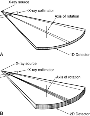
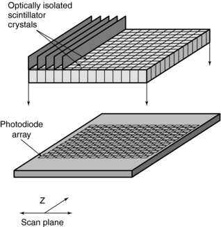
Multislice CT offers “substantial improvement of the volume coverage speed performance” (Hu, 1999a). This means that multislice CT provides faster scanning and higher resolution for a number of clinical applications (Taguchi and Aradate, 1998). One of the most conspicuous differences between multislice CT and single-slice volume CT is that the former uses a multiple row of detectors (two-dimensional [2D] detector array), whereas the latter uses a single row of detectors (1D detector array), as is clearly illustrated in Figure 12-1.

FIGURE 12-1 One of the most conspicuous differences between a single-slice volume CT scanner and a multislice CT scanner is the detector design. A, A 1D detector is used in single-slice systems. B, A 2D detector array is characteristic of multislice CT systems.

EVOLUTION OF MULTISLICE CT SCANNERS

Terminology

Several terms are used in the literature to refer to multislice CT. These include multisection CT, multidetector CT, multidetector row CT, and multichannel CT (Cody and Mahesh, 2007; Douglas-Akinwande et al, 2006). Each of these terms appears to focus on a particular outcome characteristic. For example, although the terms multislice and multisection focus on images, the terms multidetector and multidetector row focus on the detectors used during the scanning. Finally, the term multichannel refers to the function of the data acquisition system (DAS). In this textbook, the term multislice CT will be used because it has become commonplace not only in the literature but also in clinical practice (Dowsett et al, 2006; Kachelriess, 2006; Kalender, 2005).

A CT detector consists of basically two major components: a radiation sensor coupled to suitable electronics such as photodiodes and analog-to-digital converters (ADCs) (see Chapter 5). Although the radiation sensors convert x-ray photons to light, the photodiodes convert the light into electrical current (signal) that must be digitized before it is sent to a digital computer for processing. The electronics are carefully configured to the sensor elements (cells) of the CT detector and in this regard represent the data acquisition channels. As seen in Figure 12-2, the detector consists of 16 elements or cells, each 1.25 millimeters (mm) in size, and the x-ray beam is collimated to fall on four of these cells. Therefore four signals are collected per gantry rotation from each of the four cells and sent to the four ADCs to produce four slices, each 1.25 mm thick. For eight 1.25-mm thick slices, the x-ray beam would fall on eight detector elements. For four 2.5-mm thick slices, the beam would be collimated to fall on eight detector elements, where two 1.25-mm elements would be combined to produce a 2.5-mm thick slice, and so on. This electronic combination (or binning) of detector elements is described in more detail later in the chapter.

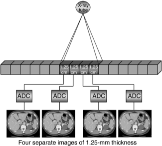
FIGURE 12-2 A diagrammatic illustration of how the detector elements from a multislice CT detector can be electronically combined to create slices of different thicknesses.

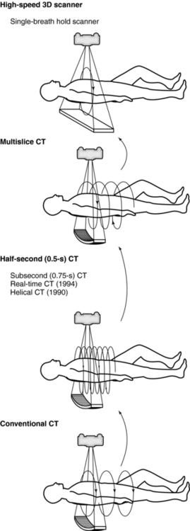
The evolution of multislice CT technology is outlined in Figure 12-3. Its overall goal is to improve volume coverage speed performance; therefore, scanning is at higher speeds with higher pitch ratios to cover large volumes with equivalent image quality compared with single-slice volume CT scanners introduced in the 1990s. The 256 CT scanner was introduced by the Toshiba Corporation Medical Systems Division as a prototype high-speed 3D CT scanner for imaging the entire heart in one complete rotation. The high-speed 3D scanner will use larger area detectors to scan larger volumes at high speeds and subsequently display all images in 3D. Finally, in 2008, Toshiba Medical Systems introduced a new 320 CT scanner. These two scanners will be described briefly later in the chapter.

FIGURE 12-3 The development continuum and milestones for Toshiba’s CT scanners.

Subsecond Scanners

Scanning time continues to decrease from the 5 minutes needed by the original EMI scanner to as low as one half second at present. The engineering barriers to be overcome in reaching this gantry speed are formidable. The acceleration on gantry components such as the tube and generator can reach 13 gravities (G), considerably more than experienced by the space shuttle at lift off. Some interesting technologic developments have accompanied the design of these high-speed CT systems.

To prevent anode movement under the stress of subsecond acceleration, new x-ray tubes have the anode mounted on a shaft that extends along the tube, providing support on both sides of the anode. This design has distinct advantages over the traditional method of supporting a massive anode from the rear only. Other innovative developments in tube design for CT include grounded anodes and a technique to reduce off-focal x-rays. Virtually all medical x-ray tubes have applied the potential difference equally between cathode and anode so that the cathode can be at 75 kilovolts (kV) while the anode is at 75 kV. This requires a substantial gap between the anode and the tube housing to reduce the possibility of arcs. With all the voltage placed on the cathode and the anode at ground potential, the tube housing can be brought into close proximity to the anode, which facilitates heat transfer and markedly improves anode cooling rate. Recoil electrons, which normally are reattracted to the anode and generate off-focal x-rays, can now be collected on a special collimator located near the anode. This eliminates off-focal x-rays that can reduce image quality and reduces the anode heat loading by about 30%, thereby reducing tube cooling delays during routine scanning.

The clinical benefits of subsecond scanning include reduced motion artifact and greater scan coverage. Patient movement during CT scanning, whether by cardiac motion, breathing, or peristalsis, may cause artifacts because filtered back-projection reconstruction combines all the views acquired during the scan rotation to cancel artifacts. Movement of any object in the field of view (FOV) during gantry rotation prevents accurate elimination of artifacts with consequent loss of image quality. If the moving object has notably high or low contrast, such as bone, calculi, or air, the artifacts are particularly noticeable. Unfortunately, the left ventricle and pulmonary vessels near the heart move so quickly that scans would have to be completed in less than 20 to 25 milliseconds to completely eliminate all blurring. This is a far shorter time than is possible with conventional CT scanners and is even difficult for electron-beam CTs, which are extremely fast. Even so, the half-second scanners, which can acquire “partial” (i.e., less than 360-degree rotation) images in 250 to 320 milliseconds have made it feasible to obtain considerably better images of the heart and chest than is possible with a 1-second system. An example is the ability of these scanners to use gated reconstruction, in which the raw scan data for image reconstruction can be selected on the basis of the patient’s electrocardiogram (ECG). Reconstruction of a gated “partial” image during cardiac diastole, when the heart is relatively quiescent, can show fairly sharp ventricular borders and calcium in the coronary arteries.

Prospective gating can also be used in which the patient’s ECG triggers the actual scan acquisition. This is a relatively simple technique, although it is not applicable to spiral/helical scanning.

A less dramatic but very practical benefit of subsecond scan times is the increased spiral/helical coverage that can become available. For the same pitch and scan duration, a half-second scanner will cover twice the anatomy that can be acquired with a 1-second scanner.

Alternatively, the half-second scanner could cover the same area by using 50% of the slice thickness, which improves z-axis resolution and leads to better image quality in 3D and multiplanar reconstructions. Clinical applications, such as CT angiography (CTA), can benefit from increased patient coverage without increasing pitch. This assumes that the system generator is able to produce enough power to accommodate the faster scans. For example, a 250-milliampere (mA) image of the abdomen requires a tube current of 500 mA in a half-second scanner.

Dual-Slice CT Scanners

The history of scanning more than one slice at a time (actually two-slice scanners) dates back to one of the early EMI (London, United Kingdom) CT scanners, which became available in 1972, and the Siemens SIRETOM (Siemens Medical Solutions, Germany) CT scanner, which appeared in 1974. These scanners used two detectors and they are based on the translate/rotate method of data collection over 180 degrees. The next major step to multislice CT scanning appeared in 1993, with the introduction of the first dual-slice volume CT scanner, the Elscint CT-TWIN (Elscint, Hackensack, NJ). The most significant difference between the dual-slice volume CT scanner and its single-slice counterpart is shown in Figure 12-4. As can be seen, the dual scanner slice geometry is based on a fan-beam of x-rays falling on two rows of detectors (Fig. 12-4, A) instead of one row of detectors, characteristic of the single-slice CT scanner beam geometry (Fig. 12-4, B).

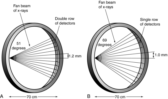
FIGURE 12-4 A, Dual scanner slice geometry based on far beam of x-rays falling on two rows of detectors. B, Single-slice CT scanner based on far beam of x-rays falling on one row of detectors.

The dual-slice whole-body fan-beam CT scanner offers improved volume coverage speed performance compared with the single-slice volume CT scanner, reducing the scan time by 50% while maintaining image quality for the same scanned volume.

Multislice CT Scanners

The dual-slice whole-body fan-beam CT technology paved the way for the development of other multislice CT scanners. These scanners were introduced at the 1998 meeting of the Radiological Society of North America in Chicago. They are based on spiral/helical scanning using multiple detector rows ranging between 8, 16, 32, 40, 64, (Kohl, 2006a), 256 (Mori et. al, 2006a), and more recently 320 (Toshiba Medical Systems, 2008) depending on the manufacturer. The 256-slice prototype scanner paved the way to the most recent commercially available multislice CT scanner, the 320 dynamic volume CT scanner. This scanner is highlighted later in the chapter.

The overall goal of the multislice CT scanner is to improve the volume coverage speed performance of both single-slice and dual-slice CT scanners. For example, a multislice CT scanner with N-detector rows (N slices) will be N times faster than its single-row (one slice) counterpart. Thus, multislice CT opens new avenues and opportunities to improve the quality of care afforded to patients because it now offers a wide range of new clinical applications afforded by recent technological developments.

PHYSICAL PRINCIPLES

Although the fundamental physics and flow of data are the same as conventional and spiral/helical CT scanners, multislice CT scanners introduce several new concepts relating to detector technology, the geometry of data acquisition, slice selection, and multislice image reconstruction algorithms.

Data Acquisition

Data acquisition is one of two mechanisms that affect image quality in CT (the other is image reconstruction). This section examines data acquisition in multislice CT with respect to beam geometry and basic parameters such as collimation, slice thickness, and pitch; but first a brief review of data acquisition in single-slice CT is in order.

Single-Slice CT: The basic data acquisition geometry for single-slice volume CT is shown in Figure 12-5. This is a third-generation scheme in which the x-ray tube is coupled to a single-row detector array positioned in the z axis.

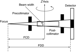
FIGURE 12-5 A side view of the basic data acquisition geometry for single-slice volume CT scanners. FCD, Focus isocenter distance; FDD, focus detector distance.

Collimation: The x-ray beam collimation system is designed to ensure a constant beam width because the precollimator and postcollimator widths are equal. The beam may or may not be collimated at the detector array. The width of the precollimator defines the slice thickness (z-axis resolution or spatial resolution) and affects the volume coverage speed performance. Although thin collimation results in better resolution and takes longer to scan a specified volume, wide collimation results in less resolution but provides better volume coverage speed. The beam width (BW) is measured in the z-axis at the center of rotation for a single-row detector array, and it is defined by the precollimator width, which determines the thickness for a single slice. A collimator width of 8 mm falling on a 1D detector array will provide a slice thickness of 8 mm.

Beam Geometry: The x-ray beam geometry for single-slice CT describes a small fan (see Fig. 12-5) and is referred to as a parallel fan-beam geometry.

Pitch: The pitch for single-slice volume CT is defined as the ratio of the distance the table translates per gantry rotation to the BW or precollimator width. As noted by Hu (1999a), “the table advancement per rotation of twice the x-ray beam collimation appears to be the limit of the volume coverage speed performance of a single-slice CT, and further increase in the table translation would result in clinically unusable images.”

Slice Thickness: In single-slice volume CT, the thickness of the slice is determined by the pitch and the width of the precollimator (which also defines the BW) at the center of rotation (see Fig. 12-5).

Multislice CT: The data acquisition geometry for multislice CT is shown in Figure 12-6 (see also Fig. 12-1, B). Perhaps the most conspicuous difference between the data acquisition geometry in Figure 12-1 and Figure 12-6 is the multirow detector array (specifically 4) coupled to the x-ray tube to describe a third-generation geometry (see Fig. 12-6, A). This 2D detector array is what Hu (1999a) refers to as the “enabling component” of a multislice CT scanner. Other important and unique features of multislice data acquisition relate to collimation, beam geometry, and pitch.

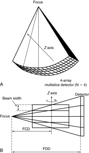
FIGURE 12-6 Data acquisition geometry for multislice CT. A, The coordinate system. B, A cross-section (side view).

Collimation: The fundamental collimation scheme is shown in Figure 12-1, B. The beam is collimated by a precollimator to fall on the entire multirow detector array. The BW is still defined in the z-axis at the center of rotation but now is for a four-row multislice detector array, as shown in Figure 12-6, B. This width will be for four slices and is prescribed by the precollimator. A precollimator width of 8 mm that falls on a four-row multislice detector array will produce four slices, each with a thickness of 2 mm (i.e., 8 mm—the total beam width in the z-axis at the center of rotation divided by 4). This is unlike the single-slice counterpart, which provides a slice thickness of 8 mm with its 8 mm wide precollimator. In addition, the four slices are a result of the division of the total x-ray beam into multiple beams, depending on the number of arrays in the 2D detector system. These multiple beams are the result of the detector row collimation or the detector row aperture (Hu, 1999a).

Figure 12-7 is a side view of a multislice CT scanner beam from the x-ray tube to the detectors. D is the width of the x-ray beam collimator and is measured at the axis of rotation; N is the number of detector rows; and d represents the detector row collimation. Hu (1999a) explains that, if the gaps between the adjacent detector rows are small and can be ignored, the detector row spacing is equal to the detector row collimation (d). The detector row collimation d and the x-ray beam collimation D has the following relationship:

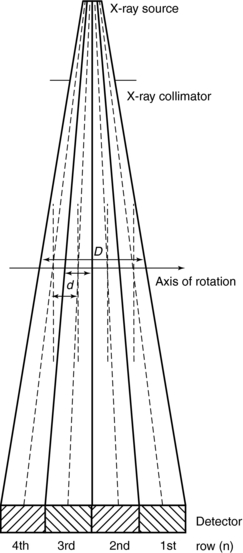
FIGURE 12-7 A side view or cross-section of a multislice CT beam geometry from the x-ray tube to a four-row multislice detector array system.

where N is the number of detector rows. In single-slice CT, the detector row collimation equals and is interchangeable with the x-ray beam collimation. “In multislice CT, the detector row collimation is only 1/N of the x-ray beam collimation.” This makes it possible “to simultaneously achieve high volume coverage speed and high z axis resolution. In general, the larger the number of detector rows N, the better the volume coverage speed performance.”

For example, if the x-ray prepatient collimation width (x-ray beam collimation) is 20 mm and the scanner has a four-row detector array, the detector row collimation is as follows:

in which d is the detector row collimation, N is the number of detector rows, and D is the x-ray beam collimator width (20/4 = 5 mm).

Alternatively,

As the beam width increases in the z direction to cover the number of rows in the 2D detector system, the amount of scattered radiation increases because a wide area of the patient is scanned. To minimize scattered radiation, antiscatter collimation may be used at the detector array (postcollimation). One such scheme is shown in Figure 12-8. Another scheme is illustrated later.

FIGURE 12-8 A proposed scheme for the use of postcollimation in multislice CT to reduce scattered radiation falling on a 2D detector array. The collimators are positioned between detector columns similar to conventional CT single-row detector arrays.

Beam Geometry: As the number of detector rows in a multirow detector array increases, the beam becomes wider to cover the 2D detector array (Fig. 12-9; see also Fig. 12-7). The beam must cover the length of the detector array. This coverage is influenced by the fan angle of the beam, in which a wider fan angle will cover a longer detector array. The beam must also cover the width of the detector array, which is defined by the number of rows in the detector array. A larger number of rows will result in a wider beam (large cone beam) in the z-axis direction.

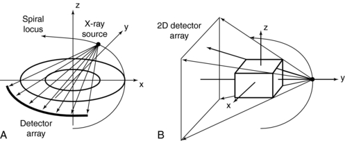
FIGURE 12-9 A, The fan-beam geometry of single-row 1D detectors, in which the rays at the detector array are almost parallel and close together. B, The concept of cone-beam geometry typical of multirow 2D detectors. The cone beam results in a wider divergence of rays at the detector array than the fan-beam geometry of single-row 1D detectors.

A cone beam geometry produces more beam divergence along the z-axis compared with fan-beam geometry. For this reason, increasing the number of detector rows in multislice CT creates a need for a different approach to the interpolation process (compared with single-slice spiral/helical interpolation) because the rays that contribute to the imaging process are more oblique. In addition, the number of detector rows plays an important role in slice thickness selection and volume coverage.

Pitch: The pitch, P, for single-slice CT is defined as the ratio of the distance, L, the tabletop travels for one complete rotation of the x-ray tube to the x-ray beam collimation. This collimation defines the BW for a single-row detector array at the center of rotation (see Fig. 12-5). The thickness of the slice is determined by the BW at the center of rotation.

In the past, the definition of pitch was somewhat varied and controversial. For example, Hu (1999a) extends the single-slice pitch definition (Equation 12-1).

(12-1)

As noted by He (1999), “the key difference here is that multislice CT beam collimation is much wider than the smallest detector row used for data acquisition. In the 4-slice scanner case, for example, one scan mode is 4 × 2.5 mm, table speed is 7.5 mm/rotation, beam width is 10 mm. So if we used our definition, the pitch value would be 7.5 mm/2.5 mm = 3. However, one could also argue that the pitch should be 7.5 mm/10 mm = 0.75. There are good arguments for either definition here.”

Taguchi and Aradate (1998) define the pitch, P, in a 4-slice scanner (four-row detector array) as:

(12-2)

where L is table speed per rotation and BW is the beam width in the z-axis for a 1-row detector array, at the center of rotation (see Fig. 12-5). For a four-slice scanner, each slice is defined by BW (see Fig. 12-6). In this case, four slices are acquired at the same time, and the helical pitch is increased by a factor of four compared with single-slice volume CT (Fig. 12-10).

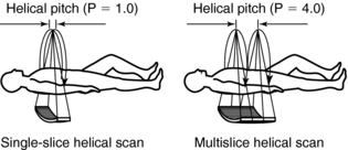
FIGURE 12-10 A comparison of the pitch between single-slice and multislice CT data acquisition. In the multislice case, the pitch is increased by a factor of 4, which allows for increased volume coverage in less time without a loss of image quality.

In addition, Kalender (2005) defines pitch for a multislice CT scanner with a four-row detector array as “the table feed, d, per full rotation relative to the slice width, S, of a single detector row (rather than relative to the total detector width).” Mathematically, this can be expressed as shown in Equation 12-3:

(12-3)

Although pitch for single-slice volume CT is defined in terms of the table speed per rotation, the definition of pitch for multislice CT is varied and is based on the table speed per rotation and either the slice thickness, the detector row collimation, or the BW at the center of rotation, depending on the manufacturer.

International Electrotechnical Commission Definition of Pitch: In 1999, the International Electrotechnical Commission (IEC) introduced a definition of pitch, which is stated in the IEC document 60601 regulation for CT, as a means of addressing the variations in definitions offered by different manufacturers (IEC, 1999). The IEC recommends the following:

(12-4)

The total collimation, on the other hand, is equal to the number of slices (M) times the collimated slice thickness (S). Algebraically, the pitch can now be expressed as follows:

(12-5)

Pitch is an important and familiar parameter in spiral/helical scanning that combines the table distance traveled per 360-degree rotation with the slice thickness. Pitch relates to the volume covered and also to patient dose. A pitch of less than 1 is effectively the same as overlapping slices and imparts a high dose. Conversely, pitches of greater than 1 result in reduced patient dose. The introduction of multislice detectors requires a reevaluation of the definition of pitch.

For a patient dose comparable to current single-slice scanners at a pitch of 1, a four-slice scanner would require a beam pitch of 1 or a slice pitch of 4. As an example, selection of 4 × 5-mm slices with a table speed of 20 mm per rotation should result in approximately the same patient dose as from a single-slice scanner operated with a 5-mm slice at 5 mm per rotation table speed. Whether this is true in practice depends on the collimator design of the specific scanner.

Slice Thickness: In multislice CT, the slice thickness is determined by the BW (see Fig. 12-6), the pitch, and other factors such as the shape and width of the reconstruction filter in the z-axis. The details of slice thickness selection for multislice CT scanners are described later in the chapter under the subsection “Slice Thickness Selection.”

Image Reconstruction

In conventional step-and-shoot CT (conventional CT), a fan-beam geometry and a single-row detector array are used in the data acquisition process, and all rays pass through the image plane (planar section), the slice of interest. With this condition, a fan-beam reconstruction algorithm, specifically, the filtered back-projection algorithm is used for image reconstruction.

Single-Slice Spiral/Helical Reconstruction: In single-slice spiral/helical CT (single-slice CT), the fan-beam geometry is maintained and a single-row detector array is used in the data acquisition process. In conventional CT, the patient is stationary during scanning, whereas in single-slice CT the patient is moving continuously through the gantry aperture during a 360-degree rotation of the x-ray tube and detectors. In this case, all rays do not pass through the image plane. A fan-beam geometry is used, so the fan-beam reconstruction algorithm used in conventional CT is used for image reconstruction. During data acquisition, the fan-beam traces a spiral/helical path around the patient, as shown in Figure 12-11. Because all rays do not pass through the image plane (planar section), single-slice spiral/helical CT requires an additional step of first calculating a planar section. This is done by interpolation, using data points on either side of the section.

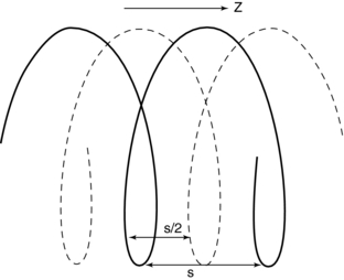
FIGURE 12-11 The spiral/helical trace of a single-row detector array in single-slice volume CT. The distance of the data points used for 360-degree LI and 180-degree LI are s and s/2, respectively.

The first interpolation algorithm used was 360-degree linear interpolation (360 degrees LI), in which the distance between the two data points used in the interpolation was represented by s in Figure 12-11. In an effort to improve the image quality resulting from the 360-degree LI, a different algorithm was developed on the basis of the mathematical fact that a CT view from a specific angle contains the same information as a view in the opposite direction (at 180 degrees). The 180-degree view, when flipped and used for interpolated reconstruction, is referred to as complementary data, as opposed to the direct, measured data. With a 180-degree LI, data points are now closer to the image plane. The distance between the two points used for interpolation is now s/2. This equation involves calculation of a complementary data set (dashed lines) using the direct fan-beam data set or measurements (solid lines). The distance between the two points used for interpolation is referred to as the z-gap (Hu, 1999a). The z-gap affects image quality so that, the smaller the z-gap, the better the image quality. In single-slice spiral/helical CT, increased volume coverage can be achieved with increased pitch; however, as the pitch increases, image quality decreases because the z-gap becomes larger. This is one motivating factor for the development of multislice CT.

Multislice Reconstruction: One of the most conspicuous differences between single-slice CT and multislice CT is that the latter uses a new detector technology in which the number of detector rows can vary from four to 320 (at the time of writing this chapter). These multiple detector rows result in a large 2D detector array. Because of this, a cone-beam geometry results instead of the fan-beam geometry characteristic of single-slice CT systems. Cone-beam geometry produces an increase in the beam divergence, which now poses a fundamental problem because all the rays do not pass through the image plane. Rays at the periphery of the beam lie outside the image plane. Approximate cone-beam reconstruction algorithms have been developed for solving this problem (Kudo and Saito, 1991); however, these particular algorithms demand extensive calculations (compared with fan-beam algorithms) and are not suitable for use in medical imaging.

Special fan-beam reconstructions (Hu, 1999a; Taguchi and Aradate, 1998) have been developed for multislice CT in its present state. In deriving an algorithm for image reconstruction in multislice CT, a logical first step is to extend the principles of 360-degree LI and 180-degree LI used in single-slice CT to multislice CT. To examine this extension, consider Figure 12-12, which shows the spiral/helical path of a four-row detector array used in multislice CT. For a 360-degree LI, the distance between the two points used for interpolation of a planar section is s, the same distance as in Figure 12-11 for single-slice CT. With a 180-degree LI, the distance of the data points is s/2 (distance between the solid and dashed lines of the same detector row). The z-gap is the same as in single-slice CT.

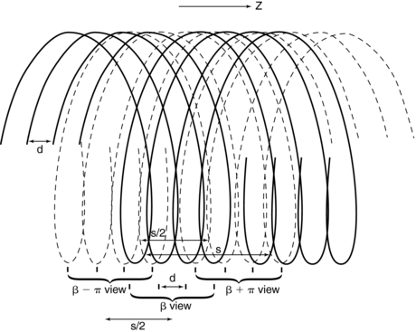
FIGURE 12-12 The spiral/helical trace of a four-row detector array in multislice CT. See text for further explanation.

Multislice CT for up to Four Detector Rows: In multislice CT, the z-gap is determined by the pitch (as in single-slice CT) and by the detector row spacing, d. “As the helical pitch varies, distinctively different z sampling patterns and therefore interlacing helix patterns may result in multislice helical CT” (Hu, 1999a). This is illustrated in Figure 12-13 for a four-row detector array for two different pitches. At a pitch of 2:1 (Fig. 12-13, A) the distance between the points used for interpolation, the z-gap, is d, “which is the same as the displacement from one solid helix to the next. This causes a high degree of overlap between different helices, generating highly redundant projection measurements at certain z-positions. Because of this high degree of redundancy (or inefficiency) in z-sampling, the overall z-sampling spacing (i.e., the z-gap of the interlacing helix pattern) is still d, not any better than its single-slice counterpart” (Hu, 1999a).

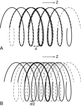
FIGURE 12-13 Spiral/helical traces for a four-row detector array in multislice CT at a pitch of 2:1 (A) and a pitch of 3:1 (B).

Increased pitch in multislice CT from 2:1 to 3:1 (Fig. 12-13, B) results in a z-gap of d/2, a much shorter distance. In this case the volume coverage speed can be increased. In addition, because the z-gap is less as the pitch increases, better image quality results. Hu (1999a) points out that “the volume coverage speed performance of the multislice scanner is substantially better than its single-slice counterpart, and so the selection of helical pitches is very critical to its performance. The pitch selection is determined by the consideration of the z-sampling efficiency and conventional factors such as volume coverage speed (which disfavors very low helical pitch); slice profile; and image artifacts, which disfavor very high helical pitch.” The preferred helical pitches are those that represent the preferred tradeoffs for various applications.

Alternatively, Figures 12-14, 12-15, 12-16, and 12-17 can be used to explain the problem and solution described previously. The unwound helical path for single-slice CT is shown in Figure 12-14 for both direct and complementary data. The image plane is interpolated using two points from the direct data and the complementary data on either side of it (image plane). Extending the single-slice concept to the multislice case as shown in Figure 12-15 results in a superimposition of the complementary and direct data for each of the detector rows in the four-row array. Note also that the z-gap is larger, and this results in image degradation. Additionally, the superimposition does not allow for efficient z-sampling. A pitch of 4 is not as preferable as a pitch of 2 because of the redundancy in the data sampling.

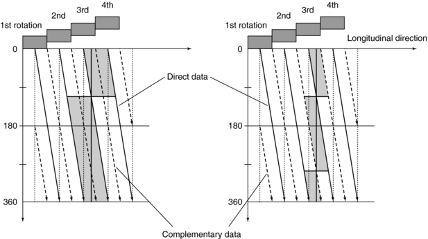
FIGURE 12-14 Single-slice spiral/helical data are generated from many gantry rotations. Reconstruction of an image in a single plane on the patient axis involves the interpolation of views in front of and behind the image plane. The use of complementary data reduces effective slice thickness but increases noise.

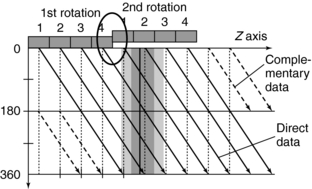
FIGURE 12-15 Rotation of a multislice detector with an even integer pitch causes the overlap of direct and complementary data from different slices. This duplication reduces the amount of information available for image reconstruction and affects image quality.

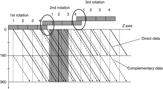
FIGURE 12-16 Careful choice of multislice pitch avoids the duplication of direct and complementary data so that image quality is not compromised.

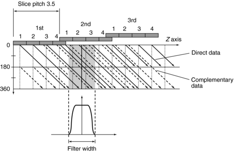
FIGURE 12-17 Filters may be used to average data along the z-axis and provide more tradeoff options between effective slice thickness and image noise to the operator.

Figure 12-16 provides a solution to the problem imposed by Figure 12-15. By separating the direct and complementary data trails, efficient z-sampling can be achieved (Saito, 1998). Taguchi and Aradate (1998) referred to this as optimized sampling scan. Figure 12-16 is with a pitch of 3.5 less than that of Figure 12-15 (pitch of 4). These figures indicate that a slight compromise in helical pitch (just 0.5) produces amazing improvement in the data sampling pattern.

The detector design for multislice CT allows the operator to select variable slice thicknesses on the basis of the requirements of the examination. The new algorithms for multislice CT also allow for the reconstruction of these variable slice thicknesses. These new algorithms address problems (image quality degradation) arising from the increase in speed (hence volume coverage) of the patient moving through the gantry aperture when the pitch is increased. Additionally, these algorithms provide for the selection of the slice thicknesses that meet the needs of the examination.

Two such algorithms were developed by Taguchi and Aradate (1998) and by Hu (1999a). These algorithms are almost identical (including the algorithm developed by Siemens Medical Systems) and are based on the same philosophy (Hu, 1999b; Taguchi, 1999).

In general, these algorithms are based on the following steps:

1. Spiral/helical scanning by interlaced sampling In this step, smaller z-gaps are obtained by adjusting or selecting the pitch to separate the complementary data from the direct data.

2. Longitudinal interpolation by z-filtering Another unique aspect of multislice data reconstruction involves averaging data in the z-axis direction. Interpolation of spiral/helical data is still needed, but the fact that the density of data points in this dimension is greater than with single-slice scanners is advantageous. One approach to image reconstruction uses a filter in the z-axis to select and weight the data points to be used in the averaging (Taguchi and Aradate, 1998) (Fig. 12-17). This is a method of a filtering process in the longitudinal (z) direction. Assuming some range with a width called the filter width (FW) in the longitudinal (z) direction (see Fig. 12-17), all data sampled within that range are processed by weighted summation. The filter parameters (e.g., FW and shape) can control the spatial resolution in the longitudinal direction, the image noise, and the image quality. Again, pitch selection is flexible and should be carefully selected. A practical advantage of this technique is that the size and shape of the filter can be selected by the operator for more control over the effective slice thickness versus noise tradeoff. As can be seen in Figure 12-17, the selection of different FWs provides considerably more control over effective slice thickness than has generally been available with single-slice spiral/helical reconstruction. FW can also substantially affect image noise compared with conventional 180- or 360-degree linear interpolation.

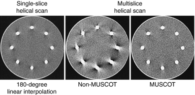
3. Fan-beam reconstruction This algorithm can be used if the number of detector rows is small. Hu (1999a) uses multiple parallel fan beams to approximate the cone-beam geometry characteristic of multislice CT. The algorithm used by Taguchi and Aradate (1998) is also based on a fan-beam method. Additionally, Saito (1998) labels the algorithm multislice cone-beam tomography reconstruction method (MUSCOT). The effect of MUSCOT on image quality is shown in Figure 12-18. Compared with single-slice CT (180-degree LI), MUSCOT provides good image quality “at a scanning speed that is about three times faster than that for single-slice CT” (Taguchi and Aradate, 1998).

FIGURE 12-18 The difference in image quality of a ball phantom obtained with a 180-degree LI algorithm (single-slice CT) and with and without the MUSCOT algorithm used for multislice CT imaging. From Saito Y: Multislice x-ray CT scanner, Med Rev 66:1-8, 1998.

Multislice CT for 16 or More Detector Rows: The previous description lends itself to multislice CT scanners with up to four detector rows. These scanners use a 2D detector array in which the x-ray beam is now opened in two dimensions to cover the entire detector array. The divergence of the beam describes a cone beam rather than a fan beam, and therefore the scanning geometry is now referred to as a cone beam. The nature and problems of using a cone beam with algorithms designed for fan-beam CT scanning geometries are outlined in Chapter 6 on image reconstruction in CT. One of the problems, for example, is related to cone-beam artifacts (streaks, for example) that degrade image quality.

The algorithms for four-slice scanners described earlier ignore the cone-beam geometry in four-slice multislice CT scanners because these algorithms assume that the measurement rays are parallel and perpendicular to the z-axis (longitudinal axis), a condition that satisfies the filtered back-projection (FBP) algorithm. Basically, the measurement rays for a planar data set are obtained by interpolation with 360-degree LI or 180-degree LI algorithms similar to those for single-slice spiral/helical CT scanners (Chapter 11), followed by the well-established and proven FBP algorithm.

As the number of detector rows increase from four to 16 to 64 and beyond, the cone beam becomes larger and cone-beam artifacts become more pronounced, especially if the object imaged is not perfectly centered in the isocenter of the CT gantry (Figure 12-19). The outer detectors receive more oblique rays compared with the central set of detectors. The effects of cone-beam geometries on image quality for these 16-slice and beyond multislice CT scanners cannot be ignored. The cone-beam angle, for example, increases by up to 16, and previous interpolation algorithms are not useful for these large cone angles (Mather, 2005a). Therefore, cone-beam algorithms are needed to address these increasing cone-beam geometries and minimize cone-beam artifacts.

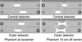
FIGURE 12-19 The appearance of streaking artifacts that occur with imaging of nonuniform objects in the z-axis with a 16-slice (cone beam) CT scanner. The artifacts are more pronounced for those created by the outer detectors and worsen if the object is not positioned accurately in the isocenter. Courtesy ImPACT Scan, London, United Kingdom.

Cone-Beam Algorithms: An Overview

Cone-beam algorithms fall into two classes, namely, (1) exact algorithms and (2) approximate algorithms. Although exact algorithms for cone-beam data have not been successful in recent times (Kalender, 2005), they are also “computationally complex and difficult to implement” (Mather, 2005a). For these reasons, they are not described in this book. On the other hand, approximate cone-beam algorithms fall into two categories: 3D algorithms and 2D algorithms (Chen et al, 2003). Two such algorithms that have become commonplace in multislice CT scanners are as follows:

1. Feldkamp-Davis-Kress (FDK), also simply referred to as the Feldkamp-type 3D algorithm

2. Advanced single-slice rebinning (ASSR) 2D approximate algorithm

Feldkamp-Davis-Kress Algorithm: The fundamental basis of the FDK algorithm is illustrated in Figure 12-20. As can be seen, the FDK algorithm simply is an extension of the 2D FBP for fan-beam geometry into a 3D FBP for cone-beam geometry (Chen et al, 2003; Kachelriess et al, 2006).

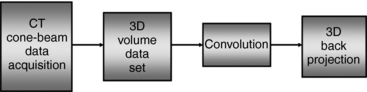
FIGURE 12-20 The most fundamental representation of the FDK algorithm for conebeam reconstruction. First, cone-beam projections of the 3D object are obtained, followed by preweighting and filtering (convolution). Finally, 3D back-projection is performed along the identical beam geometry (rays) as used for the initial cone-beam data acquisition.

This algorithm is more extensive than the 2D FBP algorithm, and it is more commonplace for use with cone-beam CT scanners (Feldkamp et al, 1984). Although the 2D FBP algorithm filters the acquired data from one-dimensional detectors, followed by a 2D fan-beam back-projection, the FDK algorithm filters the data acquired from 2D detectors (3D data set) followed by a 3D cone-beam back projection (Kalender, 2005).

There are several modifications of the FDK algorithm (referred to as Feldkamp-type algorithms) for use in multislice CT scanners; however, the principles of these algorithms are beyond the scope of this book. Two examples of these algorithms in use on some multislice CT scanners are the true cone-beam tomography (TCOT) Feldkamp-based algorithm developed by Toshiba Medical Systems, which can handle data from large cone angles, and the extended parallel back-projection (EPBP) algorithm developed by Siemens for scanners with more than 64 slices per/rotation.

A basic problem with the Feldkamp-type algorithms is that they “cannot incorporate 2D back projection hardware already available in conventional medical CT systems” (Chen et al, 2003); Kachelriess, 2006). This problem however can be solved by 2D approximate algorithms.

Two-Dimensional Approximate Algorithm: The main goal of the 2D approximate algorithms “is to provide an image quality close to that of a three-dimensional reconstruction algorithm using two-dimensional and back projection methods” (Chen et al, 2003). The principle is based on the notion of rebinning, a term used to describe the resorting of the 3D data collected from the cone-beam acquisition (geometry) to a set of 2D fan-beam projection data and subsequently use the conventional 2D FBP algorithm to reconstruct transaxial images, as illustrated in Figure 12-21.

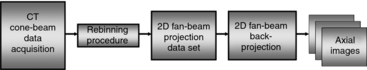
FIGURE 12-21 The basic steps of the 2D approximate reconstruction algorithm for wide cone-beam CT scanners. The acquired cone-beam data are rebinned into a 2D fan-beam projection data set that is finally back-projected by use of the 2D fan-beam reconstruction algorithm to create a set of axial images.

One early rebinning method was the single-slice rebinning (SSR) algorithm; however, it did not produce acceptable image quality for multislice CT scanners with large cone angles. Therefore, other methods were developed to solve this problem by use of a technique called tilted plane reconstruction (TPR) (Chen et al, 2003). The TPR method requires that the plane to be reconstructed is tilted (oblique) to fit the spiral/helical path of the x-ray beam to reduce cone-beam artifacts. One popular TPR algorithm is the ASSR algorithm used by General Electric (GE) Healthcare and by Siemens Medical Solutions.

The fundamental steps of the ASSR algorithm, clearly illustrated in Figure 12-22, are as follows:

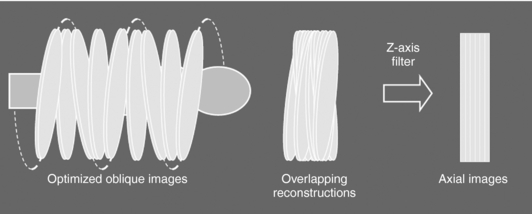
FIGURE 12-22 The basic steps of the ASSR reconstruction algorithm. See text for explanation. Courtesy ImPACT Scan, London, United Kingdom.

1. The image planes to be reconstructed make use of 180-degree segments of the spiral/helical path of the x-ray beam to obtain optimized oblique images (semicircles) because they are tilted to fit the spiral path along the z-axis of the patient.

2. The measured cone beam data are then rebinned (resorted) to produce a large number of overlapping tilted reconstruction planes that can cover the entire volume of tissue imaged.

3. In the third step, z-axis reformation (z-axis filtering) is performed to produce axial images by using the conventional 2D reconstruction algorithm on the tilted planes.

4. Finally, step 3 produces an axial image data set.

One of the fundamental problems with the ASSR algorithm is related to smaller pitch values. To solve this problem, the adaptive multiplane reconstruction (AMPR) algorithm was introduced. The AMPR algorithm is an extension of the ASSR algorithm and determines the z-axis resolution by allowing the free selection of pitch values and slice thickness (Flohr et al, 2005).

Another multislice cone-beam reconstruction algorithm that is somewhat related to the AMPR algorithm is the weighted hyperplane reconstruction (WHR) algorithm. A hyperplane is a concept in geometry. In a 2D (x, y) space, a hyperplane is a line, whereas in a 3D (x, y, z) space, a hyperplane is an ordinary plane that separates the space into two halves (OED, 2008). How this algorithm works is summarized by Flohr et al (2005) as follows: “Similar to the AMPR, 3D reconstruction is split into a series of two-dimensional reconstructions. Instead of reconstruction of traditional transverse sections, convex hyperplanes are proposed as the region of reconstruction. The increasing spiral overlap with decreasing pitch is handled by introducing subsets of detector rows, which are sufficient to reconstruct an image at a given pitch value. At a pitch of 0.5625 with a 16-slice scanner the data collected by detector rows one to nine form a complete projection data set. Similarly, projections from detector rows two to 10 can be used to reconstruct another image at the same z-axis position. Projections from detector rows three to 11 yield a third image and so on.…The final image is based on a weighted average of the sub-images.”

For a more detailed treatment of cone-beam algorithms, the interested reader should refer to the works of Kalender (2005) and Flohr et al (2005).

INSTRUMENTATION

In describing the instrumentation for multislice CT systems, it is essential to focus on the major components responsible for data acquisition, image reconstruction, image display and manipulation, image processing, image storage, recording, and image transmission.

The flow of data in multislice CT parallels that of conventional step-and-shoot CT and includes x-ray production and transmission through the patient and conversion of x-rays into electrical signals, which are subsequently converted into digital data for processing by a digital computer. Digital data in the computer are then converted into image data through image reconstruction, to be displayed on a monitor for viewing by an observer. However, the detector technology in multislice CT is one of the most significant developments in the evolution of CT. Other components of significance are the DAS and the image reconstruction system for multislice CT scanning.

The major equipment components for multislice CT are the data acquisition components, patient couch or table, the computer system, and the operator console, as shown in Figure 12-23.

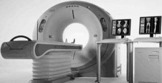
FIGURE 12-23 The major equipment components (gantry, patient couch, computer, and operator’s console) of a multislice CT scanner. Courtesy Toshiba Medical Systems.

Data Acquisition Components

The multislice CT gantry houses the x-ray generator, the x-ray tube, and detectors, as well as the detector electronics (DAS). Almost all multislice CT scanners are based on the third-generation system design, in which the x-ray tube and detectors are coupled and rotate continuously during continuous patient translation through the gantry aperture. Such data collection strategy is possible by the use of slip-ring technology (see Chapter 5).

X-Ray Generator: The x-ray generator is a compact, lightweight, high-frequency generator that provides a stable high voltage to the x-ray tube to ensure efficient production of x-rays. The power output of these generators varies depending on the manufacturer. Typical values can range from around 60 kilowatts (kW) to 90 kW.

X-Ray Tube: The x-ray tube is a rotating-anode tube capable of high heat storage capacity with high anode and tube housing cooling rates. The x-ray beam is usually fan shaped and emanates from either a small or large focal spot. X-ray tubes for multislice CT provide for a range of selectable peak kilovolts (kVp) and mAs, such as 80, 100, 120, and 140 kVp and 10 to 500 mA in increments of 10 mA. See Chapter 5 for a more detailed description of x-ray tubes, including the most recent design for use with multislice CT scanners

Multislice Detectors: Multislice detectors have evolved over time and therefore they are described in the next subsection of this chapter.

Multislice CT Detectors

The first clinical scanner, the EMI Mark 1, and several of its successors recorded two image slices simultaneously in an effort to offset their agonizingly slow scan speeds. In 1992, Elscint introduced the first modern multislice scanner, which used dual detector banks. A major difference between the EMI Mark 1 and Elscint scanners was that a particular image from the Elscint system could take advantage of data acquired by both detector banks, whereas the old EMI scanner, which predated spiral/helical acquisition, simply generated two independent images.

Detectors capable of providing more than two slices for CT scanners were introduced in 1998. At present, they allow acquisition of up to 320 slices simultaneously, and their design suggests that this number may increase in the future. This dramatic technical advance promises to have a major impact on the way CT is used in clinical practice. The tremendous increase in the rate of data collection will influence routine CT applications and create new areas for CT imaging.

Types of Detectors: As noted earlier in this chapter, the most significant difference between single-slice CT and multislice CT is the detector technology. These detectors are solid-state scintillation detectors (Fig. 12-24).

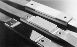
FIGURE 12-24 Examples of solid-state multirow matrix detector arrays for multislice CT scanning. These detectors are used in the GE LightSpeed QX/I CT scanner, and consist of 16 rows with 912 channels and 14,592 individual elements. Courtesy General Electric Healthcare; Milwaukee, Wis.

There are three types of detectors for use in multislice CT scanning (Cody and Mahesh, 2007; Dowsett et al, 2006; Kachelriess, 2006; Kohl, 2005). These are as follows:

1. Uniform or matrix detectors (also referred to as fixed-array detectors or linear array detectors)

2. Nonuniform or variable detectors (also referred to as adaptive-array detectors)

3. Hybrid detectors

Several different approaches to the construction of these detectors are available (Fig.12-25). As can be seen in Figure 12-25, detector arrays in the z-axis can be uniform, with all elements of the same dimensions or nonuniform to reduce the number of elements needed for thicker slices. An advantage of the nonuniform elements is the reduction of dead space (the gap between detector elements to ensure optical isolation). On the other hand, this arrangement offers less flexibility for the future, when slice numbers greater than 320 will be practical. Element dimensions shown are “effective” detector sizes, calculated at the center of gantry rotation where slice thickness is measured. The size and distribution of detector elements in the x-y plane are similar to those in current single-slice systems. Consequently, spatial or high-contrast resolution is unlikely to change significantly. Such arrays can involve more than 30,000 individual detector elements.

FIGURE 12-25 Multirow CT detector designs. Detector elements may be uniform or nonuniform. See text for further explanation.

Detector Materials: As described in Chapter 5, detectors in CT fall into two categories; gas ionization detectors and solid-state detectors. It is important to note, however, that multislice CT scanners do not use gas ionization detectors such as xenon detectors (used in the earlier single-slice CT scanners) because they have low quantum detection efficiency (<50%) and low x-ray absorption (Dowsett et al, 2006; Kachelriess, 2006; Kohl, 2005).

The detector elements of multislice CT scanners use solid-state materials (scintillation crystals or ceramics) such as cadmium tungstate and, more recently, rare earth materials such as gadolinium oxysulfide or yttrium-gadolinium oxide, gadolinium oxide, or ceramics (Dowsett et al, 2006; Kohl, 2005). The detectors are doped with suitable dopants (europium, for example) to decrease afterglow below 0.1% at 100 milliseconds (Dowsett et al, 2006).

These materials convert x-ray photons to visible light that is subsequently detected by photodiodes (see Chapter 5).

Properties of Detectors: It is beyond the scope of this text to discuss the physical properties of CT detectors; however, Dowsett et al (2006) emphasize that detectors for multislice CT scanners should have several properties. These include a large dynamic range, high quantum absorption efficiency, high luminescence efficiency, good geometric efficiency, small afterglow, and high precision machineability. In addition, they note that all detector elements must have a uniform response. Readers interested in these properties should refer to the work of Dowsett et al (2006).

Detector Configuration: The term detector configuration is a term that “describes the number of data collection channels and the effective section thickness determined by the data acquisition system settings” (Dalrymple et al, 2007). Multislice CT detectors can be configured in several ways by combining various detector elements electronically (or binning) to produce the desired slice thickness required for the examination, at the isocenter. Typical slice thicknesses that can be obtained are as follows:

• 2 × 0.5 mm, 4 × 1.0 mm, 4 × 5.0 mm, 2 × 8.0 mm, 2 × 10 mm for four-slice adaptive array detector

• 16 × 0.5 mm, 16 × 1.0 mm, 16 × 2.0 mm for a 16-slice fixed array detector

• 40 × 0.625 mm and 32 × 1.25mm for a 40-slice fixed array detector

• 64 × 0.5 mm and 32 × 1.0 mm for a 64-slice fixed array detector

The reader should consult the manufacturer data sheets for specific slice thicknesses offered by their scanners.

Slice Thickness Selection

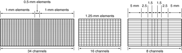
As mentioned earlier, individual slice widths (Fig. 12-26) are generally defined by the number of detector elements grouped (or binned) into each data channel (Dalrymple et al, 2007). The smallest slice width available is determined by the smallest single detector element. An exception to this generalization occurs in the nonuniform array shown in Figure 12-26, in which two 0.5-mm slices can be acquired by moving the collimator leaves inward so that only the inner half of the two central 1-mm elements are exposed to the x-ray beam. Similarly, four 1-mm slices are acquired by irradiating the two central elements and two thirds of the adjacent 1.5-mm elements. Slice width is defined at the center of rotation (center of the gantry aperture), so the actual detector dimensions for that slice will be greater because of the magnification produced by beam divergence. The x-ray beam width, as defined by the prepatient collimators, will be approximately four times the slice width.

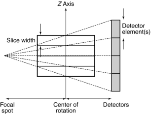
FIGURE 12-26 Slice geometry in multislice scanners. The number of detector elements grouped together determines the size of the slice. Slice width is defined at the center of gantry rotation.

The slice, as defined by the tissue irradiated during the rotation of a multislice detector, is significantly different from that of a single-detector scanner (Fig. 12-27). This is an extension of the problem with the earlier dual-detector scanners. In this case, however, the outer two slices are considerably more affected by beam divergence than are the inner two slices.

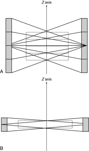
FIGURE 12-27 Comparison of slice geometry between multislice (A) and single-slice (B) scanners. The x-ray beams are shown at opposite sides of gantry rotation. Although the diagram is exaggerated, there is more beam divergence with the multislice system.

The significance of this geometric nonuniformity may be most severe in the case of conventional scanning. Reconstruction of the CT image involves all views acquired throughout the 360 degrees of data collection. When views from different angles are actually measuring quite different tissue pathways, there will be varying degrees of volume averaging with an increased likelihood of artifact and inaccurate reconstruction. If detector size is increased in future scanners to add more slices, this geometric situation will be further exaggerated. With the x-ray beam fan extended in the z-axis, as well as the x-y plane, a reconstruction algorithm that is different from those used for single-slice scanners is needed to process the raw data (Hu, 1999a; Taguchi and Aradate, 1998).

The signals from the individual detector elements are fed to four DASs through a bank of switches that combines the signals from the appropriate number of elements into the slice width selected by the operator (Fig. 12-28).

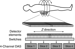
FIGURE 12-28 Switches group the signal from individual detector elements. The signals are then transferred to one of four DASs that generate the four simultaneous slices. Additional DAS channels can be added in the future.

Detector elements outside the selected slices are switched off and do not contribute any signal to the DAS. Patient dose is controlled by prepatient collimators that restrict the x-ray beam to only those detector elements needed for the four data slices. At present, the slice thickness must be selected before scanning, and it is not possible to narrow the slice width after data collection. Summing slices after scanning to create fewer, thicker images is certainly feasible and can have clinical value. In this case, it would be possible to return to the thinner slices if clinically indicated and if the raw data were still available.

Figure 12-29 provides examples of various combinations of detector elements for both fixed array and adaptive array detectors for multislice CT imaging. In addition, the detector module of a 64-slice multislice CT scanner (SOMOTOM Sensation 64, Siemens Medical Solutions, Germany) together with its antiscatter collimators (diagonally cut) is shown in Figure 12-30.

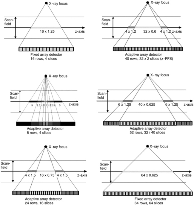
FIGURE 12-29 Examples of the use of fixed-array and adaptive-array detectors in multislice CT scanners in determining the slice thicknesses to be obtained. From Kohl G: The evolution and state-of-the-art principles of multi-slice computed tomography, Proc Am Thorac Soc 2:470-476, 2005. Reproduced by kind permission.

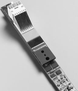
FIGURE 12-30 Photo of a detector module for the Siemens 64-slice SOMATOM Sensation multislice CT scanner showing the electronics and the antiscatter collimators that are cut diagonally (left side of the detector module). From Kohl G: The evolution and state-of-the-art principles of multi-slice computed tomography, Proc Am Thorac Soc 2:470-476, 2005. Reproduced by kind permission.

The design of the multirow detector influences the speed of acquisition of the slices and the resolution of the slices, as shown in Figure 12-31.

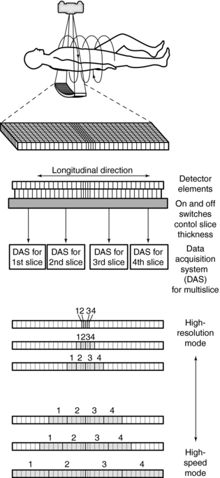
FIGURE 12-31 The multirow detector allows for various selections of slice thicknesses to meet the needs of the examination. Thinner slice thicknesses are selected in the high-resolution mode, whereas thicker slices are selected in the high-speed mode. The slice thickness is varied by turning the switches “on” or “off.”

Data Acquisition System

Another major component of the gantry is the DAS, the detector electronics responsible mainly for digitizing the signals from the detectors before they are sent to the computer for processing. Figure 12-31 shows an example of a DAS coupled to the multirow detector array by switches. In this case, four slices are acquired at the same time because of the presence of four DAS systems (four times the electrical circuits compared with single-slice CT systems) (Saito, 1998). Regardless of which four slices are required for the examination, the switches can be turned on and off to ensure that the appropriate detector segments are exposed to x-rays.

Patient Table

The patient table, or couch, features are essentially similar to those associated with single-slice CT and conventional step-and-shoot CT scanners. The purpose of the table is to support the patient and to facilitate multislice CT scanning through the variable speed of travel of the tabletop and its wide range of movement. The table can be raised and lowered to accommodate positioning of the patient in the gantry aperture and to facilitate easy transfer of the patient from the scanner to a bed or gurney and vice versa. Movement of the tabletop in the longitudinal direction also facilitates patient position in the gantry aperture, with variable scannable ranges.

Patient tables for CT are equipped with a head holder or headrest to ensure patient comfort during the examination. In an emergency during the examination, the movement of the table can be controlled manually to ensure patient safety.

Computer System

The computer system for multislice CT receives data from the data acquisition system and the operator, who inputs patient data and various examination protocols. These systems must be capable of handling vast amounts of data collected by the 2D multirow detector array. These computers have hardware architectures that provide high-speed preprocessing, image reconstruction, and postprocessing operations. Although preprocessing includes various corrections to the raw data, image reconstruction refers to the use of multislice reconstruction algorithms for image buildup. On the other hand, postprocessing involves the use of a wide range of image processing and advanced visualization software, such as the generation of 3D and MPR, as well as virtual endoscopic images from the axial data set stored in the computer.

The results of computer processing are displayed for viewing by an observer on a monitor. Several characteristics of the monitor are important to the observer, such as the display matrix, bandwidth, display memory, and the gray level and color resolution.

Data storage devices for holding the raw data and image data include hard disks, usually of the Winchester type with high storage capacities, and erasable optical disks of the magneto-optical type.

Operator Console

The operator console allows the operator to interact with the scanner before, during, and after the examination. Essentially the major components include the keyboard, mouse, monitor, and other controls for the execution of specialized functions.

The operator console controls the entire CT scanner system and facilitates the selection of scan parameters and scan control (automatic or manual), image storage, communication, image reconstruction, image processing, windowing, and control of the gantry, and x-ray tube rotation. The console allows for communication of images to other parts of the department and hospital and other remote sites through the use of local and wide area networks. The multislice CT console also supports full digital imaging and communication in medicine (DICOM) connectivity to other equipment, such as network printers, for example. Multislice CT consoles also provide for the use of a wide range of software options for image processing, such as 3D imaging, virtual endoscopy, maximum intensity projection, MPR reconstruction, cardiac applications, and dental CT and bone mineral analysis.

ISOTROPIC IMAGING

One of the major goals of developing scanners with an increasing number of slices (4, 8, 16, 32, 40, 64, 320 slices) per rotation of the x-ray tube and detectors around the patient is to achieve isotropic imaging.

Definition

Several technical developments in multislice CT scanners have made it possible to perform isotropic imaging. The term isotropic is used to refer to the size of the voxels used in a volume data set. When the slice thickness is equal to the pixel size, all dimensions of the voxel (x, y, z) are equal. In other words, the voxel is a perfect cube, and the data set acquired is said to be isotropic. If, however, all voxels dimensions are not equal, that is, the slice thickness is not equal to the pixel size, for example, the data set acquired is said to be anisotropic. The geometry of both isotropic and anisotropic data is clearly illustrated in Figure 12-32.

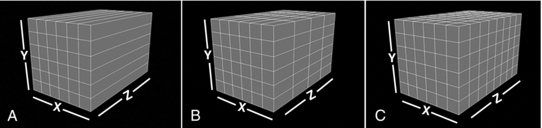
FIGURE 12-32 Geometry of isotropic and anisotropic acquisitions. Anisotropic data consist of voxels that have a section thickness greater than the x- and y-axis dimensions of the facing pixels. Section thickness along the z-axis is four times the size of each pixel in A but only twice the size of each pixel in B. Although both data sets are anisotropic, there is a significant difference in image quality for 3D applications, with improved longitudinal spatial resolution in B compared with that in A. When the section thickness is equal to the pixel size, as in C, the data are isotropic. From Dalrymple NC et al: Price of isotropy in multidetector CT, Radiographics 27:49-62, 2007. Figure and legend reproduced by permission of the Radiological Society of North America and the authors.

Goals

One of the major goals of isotropic imaging in CT is to achieve excellent spatial resolution (detail) in all imaging planes, especially in MPR and 3D imaging. In addition, there are other benefits as well (Dalrymple et al, 2007; Paulson et al, 2004, 2005), but at the expense of more dose to the patient. Furthermore, the use of narrow collimation increases the scanning time. As noted by Dalrymple et al (2007), “the parameters that affect the radiation dose and exposure time vary considerably according to scanner design and these variations determine the proportions of the trade-off in increased radiation dose and scanning time relative to the voxel size.” Therefore, in MSCT scanning, personnel should have a working knowledge of how voxel size affects not only the spatial resolution but also the radiation dose. Such understanding ensures that personnel work within the ALARA (as low as reasonably achievable) philosophy to optimize the image quality and radiation dose.

Data Acquisition

Isotropic imaging with 4-, 16-, 40-, and 64-channel multislice CT scanners has been described in some detail by Dalrymple et al (2007). One of the major technical parameters that have an effect on isotropy is the detector configuration, that is, how the detector elements are used together with the effective slice thickness. Although the four-channel multislice CT scanner can achieve near isotropic imaging, the 16-, 32-, 40-, and 64-channel multislice CT scanners can produce isotropic voxels, hence achieve isotropy. As demonstrated by Dalrymple et al (2007), the scanners (beyond four-slice) can also produce voxels that are anisotropic.

The detector configurations and voxel dimensions for isotropic and anisotropic imaging are illustrated in Figure 12-33, A, for a 16-channel CT scanner and in Figure 12-34, A, for a 64-channel CT scanner. The fundamental principles for isotropic reconstructed voxels are shown in Figures 12-33, A, and 12-34, A, and anisotropic reconstructed voxels are illustrated in Figures 12-33, B, and 12-34, B. The effects of isotropic data acquisition and anisotropic data acquisition on 3D volume-rendered images are shown in Figure 12-35 and Figure 12-36 for 16- and 64-channel CT scanners, respectively.

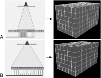
FIGURE 12-33 Detector configurations and voxel dimensions at 16-channel multidetector CT. A, Left, Diagram shows narrow collimation, with exposure of only the central 16 detector elements. Each element functions as a separate unit, and 16 sections with a thickness of 0.625 mm each are acquired per gantry rotation. Right, Diagram shows that the reconstructed voxels are isotropic, with about equal length in each dimension. B, Left, Diagram shows wide collimation, with exposure not only of the central small elements but also of larger elements at the periphery. Central elements function in pairs, and peripheral elements are used individually. As a result, 16 sections with a thickness of 1.25 mm each are acquired per rotation. Right, Diagram shows that reconstructed voxels are anisotropic, about twice as long in the longitudinal plane as in the transverse plane. From Dalrymple NC et al: Price of isotropy in multidetector CT, Radiographics 27:49-62, 2007. Figure and legend reproduced by permission of the Radiological Society of North America and the authors.

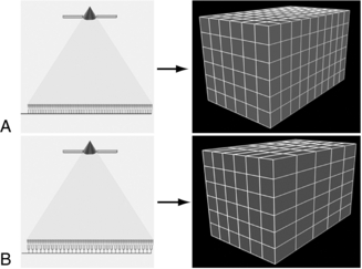
FIGURE 12-34 Detector configurations and voxel dimensions at 64-channel multidetector CT. Because the width of the incident beam does not change between detector configurations, the concepts of narrow and wide collimation do not apply. A, Left: Diagram shows the detector configuration for thin-section acquisitions. With each detector element used individually, 64 sections with a thickness of 0.625 mm each are acquired per gantry rotation, resulting in long-axis coverage of 40 mm. Right: Diagram shows that reconstructed voxels in this mode are isotropic, with approximately equal length in each dimension. B, Left: Diagram shows the detector configuration for acquisition of thicker sections. Although the beam collimation does not change, the data acquisition system pairs the elements for the receipt of data. As a result, 32 sections with a thickness of 1.25 mm each are acquired per gantry rotation, while long-axis coverage remains constant. Right: Diagram shows that reconstructed voxels in this mode are anisotropic, approximately twice as large in the longitudinal plane as in the transverse plane. From Dalrymple NC et al: Price of isotropy in multidetector CT, Radiographics 27:49-62, 2007. Figure and legend reproduced by permission of the Radiological Society of North America and the authors.

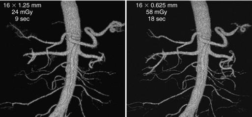
FIGURE 12-35 Three-dimensional volume-rendered images from renal CT angiography with a 16-channel scanner. The first row of data on the images is the detector configuration, the middle row is the volume CT dose index, and the bottom row is the scanning time. A, Image reconstructed from anisotropic data provides satisfactory depiction of the aorta and central vessels. B, Image reconstructed from isotropic data provides slightly improved definition of smaller vessels. The automated “seed and grow” software program used to create these images provided better depiction of peripheral branches of the renal vessels with the use of isotropic data. From Dalrymple NC et al: Price of isotropy in multidetector CT, Radiographics 27:49-62, 2007. Figure and legend reproduced by permission of the Radiological Society of North America and the authors.

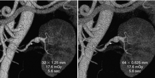
FIGURE 12-36 Volume-rendered images from 64-channel multidetector CT. The first row of data on the images is the detector configuration, the middle row is the volume CT dose index, and the bottom row is the scanning time. A, Image reconstructed from anisotropic data (section thickness, 1.25 mm; increment, 0.625 mm) clearly depicts a peripheral aneurysm of the left renal artery. B, Image reconstructed from isotropic data (section thickness, 0.625 mm; increment, 0.3 mm) provides sharper definition of vessel margins and allows visualization of small lumbar and mesenteric vessel branches. From Dalrymple NC et al: Price of isotropy in multidetector CT, Radiographics 27:49-62, 2007. Figure and legend reproduced by permission of the Radiological Society of North America and the authors.

IMAGE QUALITY CONSIDERATIONS

Image quality in CT is described in detail in Chapter 9. Essentially there are three main parameters: spatial resolution, contrast resolution, and noise. Spatial resolution, the ability of the scanner to image fine detail, is measured in line pairs per centimeter. Contrast resolution or low-contrast resolution or tissue resolution is the ability of the scanner to discriminate small differences in tissue contrast. Noise, on the other hand, is a fluctuation of CT numbers from point to point in the image for a scan of uniform material such as water. Noise degrades image quality and affects the perceptibility of detail. Artifacts can also degrade image quality and cause problems in image interpretation.

In multislice CT, these parameters are the same in terms of definition. Recall that the purpose of multislice CT is to improve on the performance of single-slice CT in terms of speed and coverage. The volume coverage speed performance in multislice CT is better than its counterpart single-slice CT without compromising image quality.

In addition, image quality depends on radiation dose. Although the dose in CT has received increasing attention in the literature and has been identified as an increasing source of radiation exposure and may be viewed as “a public health issue in the future” (Brenner and Hall, 2007), there have been increasing technical efforts to reduce this dose not only to adults but to children in particular. One such dose reduction technology is the tube current modulation techniques introduced by manufacturers. Dose in CT is described in detail in Chapter 10.

Acceptance testing and research studies will provide verification on image quality parameters and more information on the performance of multislice CT scanners in the image quality and radiation dose arenas.

BEYOND 64-SLICE MULTISLICE CT SCANNERS: FOUR-DIMENSIONAL IMAGING

Limitations of Previous Multislice CT Scanners

The technical evolution of multislice CT scanners from 16-slice, 32-slice, 40-slice, and 64-slice CT scanners has resulted in numerous clinical benefits not only to enhance diagnosis but also for use in radiation therapy and surgical simulation, for example. One such benefit of multislice CT imaging is improved 3D imaging of anatomical structures. It is still a problem, however, to obtain dynamic 3D images of the beating heart in cardiac imaging, for example. Dynamic 3D is referred to as four-dimensional imaging (Mori et al, 2004). In addition, these multislice CT scanners can increase the dose to patients (Brenner and Hall, 2007), create image artifacts especially in cardiac CT imaging as a result of the beating heart, and have limited organ coverage because of the size of the detector (20-40 mm). The latter implies that two or more rotations are needed to cover the entire organ, such as the heart or lungs. To solve these problems, two other multislice scanners have been developed and are being implemented into clinical practice. These two scanners are the 256-slice and 320-slice CT scanners.

The 256-Slice Beta Four-Dimensional CT Scanner

The first model of the 256-slice 4D CT scanner was developed at the National Institute of Radiological Sciences in Japan in 2003. The major goal of this scanner is to produce four-dimensional CT images with a wide-area detector capable of covering the entire organ (heart or lung) in a single rotation rather than multiple rotations.

The second model of the 256-slice four-dimensional CT scanner (Fig. 12-37, A) is based on the design of the first model, and in 2006 and 2007 this model prototype scanner was installed in three centers for clinical beta trials. These centers include the Fujita Health University in Nagoya, Japan; the National Cancer Center in Tokyo, Japan; and Johns Hopkins University in Baltimore, Maryland.

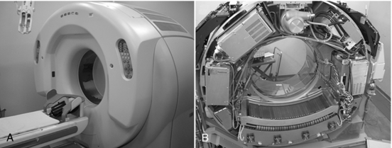
FIGURE 12-37 The second model of the 256-slice beta four-dimensional CT scanner showing the external gantry and table in A and the x-ray tube, wide area detector, and associated electronics mounted on the rotating frame of the gantry. A, Courtesy Shinichiro Mori, Radiological Protection Section, National Institute of Radiological Sciences, Japan. B, Courtesy Toshiba Medical Systems.

The most conspicuous difference is the use of a wide-area 2D detector mounted on the gantry frame of a 16-slice CT scanner (Aquilion, Toshiba Medical Systems, Tokyo Japan), as shown in Figure 12-37, B. The scanner uses a cone beam with a larger cone angle (about 13 degrees) compared with the previous multislice CT scanners to cover a wider FOV. The total beam width is 128 mm, four times the size of the Aquilion 16-slice CT scanner (Toshiba Medical Systems). This wide beam ensures complete coverage of the entire organ (heart) in one complete rotation (Fig. 12-38).

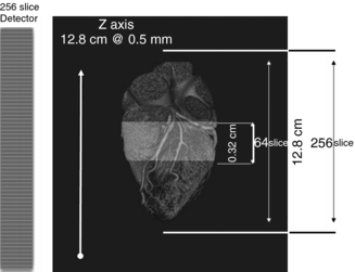
FIGURE 12-38 The wide area detector of the 256-slice beta four-dimensional CT scanner ensures coverage of the entire heart with one complete rotation. Courtesy Toshiba Medical Systems.

The 256-slice four-dimensional CT scanner has 912 (transverse) × 256 (craniocaudal) detector elements, each approximately 0.5 mm × 0.5 mm at the center of rotation. The 128-mm total BW allows for the continuous use of several collimation sets. The detector element is made of a gadolinium oxysulfide (Gd₂O₂S) and a single crystal silicon photodiode as used in the current multislice CT scanners.

The rotation time is 0.5 seconds per rotation and the dynamic range is 18 bits. The reconstruction algorithm used in this scanner is the Feldkamp cone-beam algorithm. Real-time reconstruction processing is done by 32 field programmable gate arrays (FPGSs-Virtex II Pro, Xilinx, San Jose, Calif.) with a clock speed of 125 megahertz. Volumes of 256 × 256 × 128 can be produced.

The clinical beta testing program of the 256-slice CT scanner laid the foundations for the design of a new multislice CT scanner designed to image the entire heart, for example, in a single rotation. This scanner is Toshiba’s 320-slice Aquilion ONE Dynamic Volume CT scanner (Toshiba Medical Systems), which is described briefly in the next section.

The 320-Slice Dynamic Volume CT Scanner

In 2007, the 320-slice CT scanner referred to as the AquilionONE MSCT scanner (Fig. 12-39) was introduced at the Radiological Society of North America meeting in Chicago. One of the characteristic technical features of this scanner is its wide-area 2D detector that ensures a field coverage of 160 mm (compared with 128 mm of the 256-slice prototype CT scanner). The detector design is such that the number of detector rows is 320 ultrahigh resolution detector elements. This feature allows for scanning the entire anatomical structures such as the heart, lungs, and brain, in a single rotation and therefore not requiring the spiral/helical scanning principle.

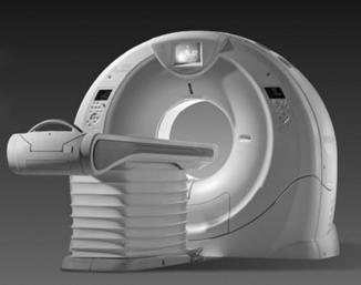
FIGURE 12-39 The gantry and patient table of the 320-slice dynamic volume CT scanner. Courtesy Toshiba Medical Systems.

This high-speed volume scanner features a rotation time of 350 milliseconds, which is needed to provide a temporal resolution for imaging the entire heart in one heartbeat with excellent spatial and contrast resolution at lower doses (Mather, 2007). In addition, the reconstruction time is fast (less than 10 seconds) and is made possible through the use of specially designed reconstruction processors.

A major challenge in the development of this wide area detector CT volume scanner is the large cone angle because the beam divergence is much greater than that of the 256-slice scanner. To address this problem, Toshiba developed an FDK-based algorithm called the coneXact reconstruction algorithm to eliminate any cone-beam image artifacts.

The 320-slice volume scanner can be used in neurological imaging, cardiac imaging, and other body applications where entire organs (chest, for example) can be scanned very quickly. Such scanning results in large data sets that will provide more information for the radiologist to use in diagnostic management of the patient.

BEYOND SINGLE-SOURCE MULTISLICE CT SCANNERS: Dual-Source CT Scanner

In 2006, a CT scanner primarily for cardiac imaging (and other applications as well) was introduced at the Radiological Society of North America meeting. This scanner, the dual-source CT scanner introduced by Siemens Medical Solutions (Forchheim, Germany), featured a unique design incorporating two x-ray tubes coupled to two detector systems that in this manner provided a scanner with two DASs.

CT imaging of the heart with multislice CT scanners dates back to 1999 and, because the heart is in constant motion (beating heart), temporal resolution is essential to avoid motion artifacts. Additionally, for cardiac imaging with CT, it is important to cover the entire heart in a single breath-hold. Although four-slice CT scanners provided acceptable results, problems with respect to motion artifacts, greater heart rates, long breath-hold times, and limited spatial resolution still persist (Flohr et al, 2006).

The introduction of 16-slice scanners provided improved gains in spatial and temporal resolution compared with four-slice systems. The subsequent arrival and use of 64-slice CT scanners provided further improvements in the technical requirements for cardiac imaging. For example, these scanners provided spatial resolution (by isotropic imaging) and temporal resolution because of the reduction of gantry rotation times to 0.33 milliseconds (necessary to deal with high rates) compared with about 0.375 seconds for 16-slice scanners (Flohr et al, 2006). One of the problems in CT cardiac imaging is to remove the need for heart rate control, and therefore efforts are needed to improve temporal resolution below 100 milliseconds at any heart rate.

To solve these problems, other scanners are needed. One such scanner that was developed was the electron beam CT scanner (see Chapter 5). Although this scanner provided some benefits in imaging (for example, the scanner does not have any moving parts), it did not provide a sufficient signal-to-noise ratio when imaging large patients. Therefore, this scanner “is currently not considered adequate for state-of-the-art cardiac CT imaging or for general radiology applications” (Flohr et al, 2006).

In an effort to further improve the temporal resolution needed for cardiac CT imaging by a factor of 2 (Cody and Mahesh, 2007, and see reference 3 in Cody and Mahesh), another CT scanner, the dual-source CT scanner, dedicated to cardiac imaging, developed by Siemens Medical Solutions, was called the Definition (Forchheim, Germany). The design concept of the scanner is based on the use of two x-ray tubes coupled to two separate detector systems, as mentioned earlier.

Major Technical Components

The major system components of the dual-source CT scanner are illustrated in Figure 12-40. The most noticeable difference between this scanner and other multislice CT scanners is that there are two data acquisitions systems offset by 90 degrees (Engel et al, 2008). Although an acquisition system labeled “Det A” has a scan (FOV coverage of 50 centimeters in diameter, an acquisition system labeled “Det B” is smaller in size compared with “Det A” and has a smaller scan FOV diameter of 26 centimeters. This reduction in size of one acquisition system is due to the restricted space in the gantry.

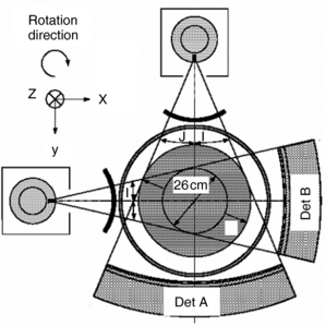
FIGURE 12-40 The major components of the dual-source CT scanner, which consists of two DASs, that is, two x-ray tubes coupled to two separate detector systems, Det A, which covers the entire scan field-of-view (scan FOV = 50 cm in diameter); and Det B, which covers a smaller central scan FOV (26 cm in diameter). See text for further explanation. From Flohr TG et al: First performance of a dual-source CT (DSCT) system, Eur Radiol 16:256-268, 2006. Reproduced by kind permission.

Each x-ray tube is of the STRATON type (Siemens Medical Solutions, Forchheim, Germany) that uses the z-flying focal spot technique (see Chapter 5) and cone-beam geometry to image two 32-slices (0.6 mm) combined to produce 64 slices per revolution. The detectors are multislice detectors with 40 detector rows of the hybrid design where the central 32 rows would produce a 0.6-mm slice width and the two outer rows provide slice widths of 1.2 mm. In addition, each x-ray tube can be operated separately with regard to the exposure technique (kVp and mA). This feature allows the scanner to perform dual-energy imaging, where one tube can operate at say 80 kVp and the other at say 140 kVp (Flohr, 2006).

Cardiac Imaging with the Dual-Source CT Scanner

The dual-source CT scanner is primarily “well-suited” for cardiac imaging for several reasons (Cody and Mahesh, 2007), an important reason being that the design of the system offers excellent temporal resolution compared with other multislice CT scanners. Such resolution is needed to reduce motion artifacts created by the beating heart. Although it is not within the scope of this text to describe the details of cardiac CT imaging, the following points (from several experts) about the DSCT scanner are noteworthy:

1. “Because the minimum rotation speed required for a cardiac CT image is equal to just over one-half of a rotation for a conventional multislice CT scanner, it is also equal to just over one-fourth of a rotation for a dual-source MSCT scanner” (Cody and Mahesh, 2007).

2. The dual-source CT scanner improves the temporal resolution for cardiac CT imaging by a factor of 2 (Cody and Mahesh, 2007).

3. “In a single detector row spiral CT, noise is independent of pitch. Conversely in non-cardiac multi-detector row CT, noise depends on pitch because the spiral interpolation algorithm makes use of redundant data from different detector rows to decrease noise for pitch values less than 1 (and increase noise for pitch values >1. However, in cardiac CT, redundant data cannot be used because such data averaging would degrade the temporal resolution” (Primak et al, 2006).

4. “In addition, linking the heart rate to the pitch (by which a higher rate can be examined by using a higher pitch), effectively reduces the dose to radiation delivered during the examination and can also eliminate the need for additional drugs (e.g., β-blockers) before the cardiac CT examination to reduce the heart rate” (Cody and Mahesh, 2007).

5. “The minimum amount of data required to reconstruct a CT image is 180° plus the angle (in degrees) of the x-ray beam in the plane of the image (known as the fan angle). Hence cardiac algorithms use partial reconstruction technique (180° + the fan angle) to reconstruct an image. These data are collected either during a single cardiac cycle (single segment reconstruction) or during two or more consecutive heartbeats (multi-segment reconstruction). In both cases the number of photons N contributing to the cardiac reconstruction depends only on the tube current and time it takes the gantry to rotate through 180°⁰ plus the fan angle, and not the pitch” (Primak et al, 2006). Because faster rotation times require lower pitch values in cardiac multidetector row CT, dose is increased without a commensurate decrease in noise (Primak et al, 2006).

6. “Several steps can be taken to reduce the dose, including lowering the tube current as the x-ray beam crosses over certain areas of the body; decreasing the tube current during certain phases of the cardiac cycle, and using a higher pitch” (Primak et al, 2006).

Other Imaging Applications

Other applications of the dual-source CT scanner include the following:

1. Imaging obese patients. Because the dual-source CT scanner can operate at a higher power rating (higher kW) compared with the lower kW power rating of a single-source CT scanner by using the power of two x-ray tubes, better image quality for obese patients can be obtained.

2. Dual-energy imaging. The dual-source CT scanner overcomes the problems of dual-energy imaging afforded by the earlier CT scanners. The two x-ray tubes can be operated at two different kVp values, producing images with different tissue characterization, because the absorption of x-rays in tissues depends on the kVp of the beam used. For example, scanning at 80 kVp, the CT number for bone and iodine are 670 Hounsfield units (HU) and 296 HU, respectively. At 140 kVp, the CT numbers for bone and iodine are 450 HU and 144 HU, respectively (Siemens Medical Solutions, 2006). This difference is useful in CTA, where it is necessary to separate bone from vessels filled with iodine.

3. Finally, the dual-source CT scanner can perform in a similar manner as a single-source 64-slice CT scanner by using only one acquisition system (one x-ray tube coupled to a detector array) (Siemens Medical Solutions, 2007).

ADVANTAGES OF MULTISLICE CT

The advantages of multislice CT have been outlined by Saito (1998) and Cinnamon (1998), as well as by Kohl (2005), Kalender (2005b), Mather (2005b), Douglas-Akinwande (2006), Kachelriess, (2006), and Cody and Mahesh (2007). There are several factors in multislice CT scanning that combine to improve not only the spatial and contrast resolution of images but also the temporal resolution (fewer motion artifacts) as well. Furthermore, multislice CT opens up improved gains in other clinical applications such as improved MPR images and 3D rendered images, retrospective creation of thinner or thicker sections from the same raw data, and delivery of intravenously administered iodinated contrast material at faster rates, and so on.

Essentially, these advantages include the following:

1. Increase in speed and volume coverage. In multislice CT, the increase in pitch and the increase in rotation speed of the x-ray tube and detectors allow for a larger volume of the patient to be scanned in less time. Hu (1999a), for example, showed that a four-slice helical/spiral CT scanner is about two times faster than a single-slice CT scanner for comparable image quality.

2. Improved spatial resolution. Multislice CT images thin slices with better isotropic resolution. This is sometimes referred to as isotropic imaging, in which case all the sides (axial, vertical, and horizontal) of the voxels in the slice have equal dimensions compared with single-slice CT. This advantage provides improved MPR and 3D images with reduced image artifacts.

3. Efficient use of the x-ray beam. In multislice CT, the x-ray beam width has to be opened to fall on the 2D detector array compared with a single-row detector array characteristic of single-slice CT scanners. The entire beam is thus used to acquire four slices (images) per 360-degree rotation without wasting any portion of the x-ray beam, as opposed to one slice per 360-degree rotation in the single-slice CT case, in which a portion of the x-ray beam is wasted during data acquisition. Such use of the beam increases the life of the x-ray tube. The tube can now be used to produce a large number of thin slices without having to wait for it (x-ray tube) to cool, a problem with single-slice CT systems. In 1999, Kopecky et al (1999) noted that with an x-ray tube with a lifespan of 200,000 seconds, a single-slice CT scanner will provide about 200,000 image (one image/second) compared with 800,000 images for a four-slice multislice CT scanner (same conditions are maintained), “or 1.6 million images if the gantry spins at two revolutions per second, or 3.2 million images if two images are created for each full rotation of 0.5 secs.”

4. Reduction of radiation exposure. The development of new dose reduction technology, such as for example, tube current modulation techniques, will play a significant role in CT dose reduction.

5. Improved accuracy in needle placement in CT fluoroscopy. One of the problems with needle placement under CT fluoroscopic control with a single-slice CT scanner is illustrated in Figure 12-41. The image shows that the needle has hit the target, which is simply not the case. This problem is solved with multislice CT scanners that offer CT fluoroscopy because multiple images are obtained. It is apparent in Figure 12-41 that the target has been hit.

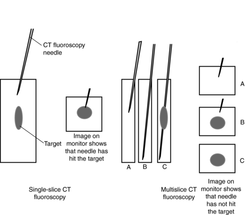
FIGURE 12-41 A comparison of the accuracy of needle placement in CT fluoroscopy from single-slice CT and multislice CT systems.

6. Cardiac CT imaging. Multislice CT technology has been developed to such a level that “dedicated” CT scanners for imaging the heart such as the dual-source CT scanner and the 320-slice four-dimensional CT scanner are now available commercially. These scanners can image the heart (and other organ systems) with exceptional spatial, contrast, and temporal resolution, as well as with reduced doses compared with 64-slice CT scanners. Additionally, the use of special cardiac reconstruction algorithms can have an impact on artifact reduction when the beating heart is imaged (Cody and Mahesh, 2007; Dowe, 2006; Flohr, 2006; Flohr et al, 2006; Kachelriess, 2006; Mather, 2005b; Mather, 2007; Primak et al, 2006).

CLINICAL APPLICATIONS

The immediate advantages of multislice CT are the speed of volume acquisition and the reduced loading on the x-ray tube. The same anatomic coverage may be obtained in one fourth the time and at one fourth the anode heating with all other parameters remaining the same. The implications for the x-ray tube are enormous. Not only is it possible to perform many more acquisitions before the necessary pause for tube cooling, but the wear and tear on the tube is also greatly reduced for the same scan volume. For example, a full-body scan from head through the pelvis, which would require more than 95 seconds of data collection in a 1-second, single-slice scanner (excluding interscan delays), could be performed in less than 12 seconds of data collection for a half-second multislice system.

Such amazing speed should have immediate value in examinations of trauma and pediatric patients. Better phase differentiation in contrasted studies is now possible, which hopefully will lead to improved diagnostic information. However, just as the introduction of spiral/helical CT emphasized the need for accurate contrast timing, the speed of multislice scanning will make this accuracy even more critical. Accurate contrast tracking techniques such as those available from continuous imaging technology will play an even greater role in the optimization of contrast opacity in both routine and special examinations.

As with spiral/helical scanning, speed may be exchanged for improved image quality. With the single-slice scanner, technique selection must balance the volume to be covered against slice thickness and pitch. Multislice systems offer the possibility of extended coverage with thin slices, which improves z-axis resolution and reduces partial volume averaging. These effects should be particularly noticeable in 3D and MPRs of scan data in CT angiography, for example.

It has been demonstrated that, for example, 0.5-mm slices can be achieved in reasonable scan times, which brings isotropic resolution in 3D reconstructions within reach. This is particularly valuable in cerebral CT angiography for the more accurate visualization of small vessels. Aneurysms and stenoses may be characterized quantitatively to yield better diagnostic information and allow the presurgical preparation of customized stents and other devices for more effective therapy. Similar improvements in CTA of the neck, aorta, and renal vessels are available with these scanners because of the combination of speed and thin slices for high axial resolution. Indeed, examples of peripheral runoff studies are appearing in which superb CT angiograms of the aorta and lower extremities can be completed in 75 seconds with substantially less contrast volume. In addition to more accurate CT angiography, the ability to cover large volumes with excellent spatial resolution should also provide more accurate data sets for the performance of CT endoscopy and the diagnosis of pulmonary embolism.

Another exciting prospect with multislice detectors is the continued development of functional CT imaging. Examples of the usefulness of CT in the evaluation of perfusion and other functions in various parts of the body have been reported. Now that a larger volume of data can be continuously acquired, the potential of CT in functional studies has been fully realized. An application of this technique is the evaluation of brain perfusion through the observation of first-pass contrast flow in patients suspected of acute infarction.

Clinical applications are discussed further in Chapters 17, 18, and 19.

POTENTIAL PROBLEMS

Although multislice scanners offer dramatic advantages compared with their single-slice counterparts, they also have some potential problems. Cases that are currently scanned with thin slices, overlapped reconstruction, and possibly two or more reconstruction algorithms can generate huge numbers of images. Routine studies consisting of hundreds of images are common, and special examinations might involve thousands of images. Obviously, such large data sets present problems for interpretation, recording, distribution, and archiving. Radiologists are now making the diagnosis from “soft” reading of images on workstations, and are reading MPR and 3D reconstructions instead of individual axial images. Reliance on remote locations for diagnosis may strain existing transmission capabilities and necessitate considerably faster systems for the future.

It will no longer be practical to record all CT images on film, and even archiving to digital media may require new strategies such as “stacking” slices or selective archival. Some departmental PACS (picture archiving and communication systems) have already been stretched beyond their capabilities by the flood of new data, and great care is needed in future facility design. The handling of image data may be the next big problem area for CT.

REFERENCES

Brenner, DJ, Hall, EJ. Computed tomography—an increasing source of radiation exposure. New Engl J Med. 2007;357:22.

Chen, L, et al. General surface reconstruction for cone-beam multislice spiral computed tomography. Med Phys. 2003;30:2804–2812.

Cody, DD, Mahesh, M. Technologic advances in multislice CT with a focus on cardiac imaging. Radiographics. 2007;27:1829–1837.

Dalrymple, NC, et al. Price of isotropy in multidetector CT. Radiographics. 2007;27:49–62.

Daly, B, Templeton, PA. Real-time CT fluoroscopy: evolution of a clinical tool. Radiology. 1999;211:309.

Douglas-Akinwande, AC, et al. Multichannel CT: evaluating the spine in postoperative patients with orthopedic hardware. Radiographics. 2006;26:S97–S110.

Dowe, DA. Prospectively gated CTA dramatically reduces dose. Diagn Imaging. 2006;28:S1–S5.

Dowsett, D, et al. The physics of diagnostic imaging. London: Hodder Arnold, 2006.

Engel, KJ, et al. X-ray scattering in single- and dual-source CT. Med Phys. 2008;35:318–332.

Feldkamp, LA, et al. Practical cone-beam algorithm. J Opt Soc Am. 1984;1:612–619.

Flohr, TG, et al. Multi-detector row CT systems and image reconstruction techniques. Radiology. 2005;235:756–773.

Flohr, TG. Radiation dose with dual source CT. Siemens Med Solutions. 2006:94–97. [June].

Flohr, TG, et al. First performance of a dual-source CT (DSCT) system. Eur Radiol. 2006;16:256–268.

He HD: Personal communication, General Electric Medical Systems, 1999.

Hu, H. Multislice helical CT: scan and reconstruction. Med Phys. 1999;26:5.

Hu H: Personal communications, 1999b.

IEC (International Electrotechnical Commission): Medical Electrical Equipment-60601 Part 2-44: Particular requirements for the safety of x-ray equipment for computed tomography, Geneva, Switzerland, 1999.

Kachelriess, M, et al. Extended parallel backprojection for standard three-dimensional and phase-correlated four dimensional axial and spiral cone-beam CT with arbitrary pitch, arbitrary cone angle, and 100% dose usage. Med Phys. 2004;31:1623–1641.

Kachelriess, M. Clinical x-ray computed tomography. In: Schlegel W, et al, eds. New technologies in radiation oncology. New York: Springer, 2006.

Kalender, WA. Computed tomography: fundamentals, system technology, image quality, applications. Erlangen, Germany: Publicis Corporate Publishing, 2005.

Kalender, WA, Kyriakou, Y. Flat-detector computed tomography (FD-CT). Eur Radiol. 2007;17:2767–2779.

Kohl, G. The evolution and state-of-the-art principles of multi-slice computed tomography. Proc Am Thorac Soc. 2005;2:470–476.

Kopecky, K, et al. Multislice CT spirals past single-slice in diagnostic efficacy. Diagn Imaging. 1999:36–42. [April].

Kudo H, Saito T: Helical-scan computed tomography using cone-beam projections. In IEEE Conf. Record 1991 Nuclear Science Symposium and Medical Imaging Conference, Santa Fe NM, 1958-1962, 1991.

Liang, Y, Kruger, RA. Dual-slice spiral versus single-slice spiral scanning: comparison of the physical performance of two computed tomography scanners. Med Phys. 1996;23:205–217.

Mather, R. Meeting the cone-beam challenge— Aquilion’s ^sureCardio^TM and TCOT. Toshiba Med Rev. 2005;15:16–21. [October].

Mather, R. Patient focused imaging—Aquilion’s low dose vision. Toshiba Med Rev. 2005;17:4–8. [July].

Mather, R. Aquilion ONE—dynamic volume computed tomography. Toshiba Medical Systems, 2007.

Meyer, CA, et al. Real-time CT fluoroscopy: utility in thoracic drainage procedures. AJR Am J Roentgenol. 1998;171:1097.

Mori S: Personal communications, 2008.

Mori, S, et al. Physical performance evaluation of a 256-slice CT-scanner for four-dimensional imaging. Med Phys. 2004;31:1348–1356.

Mori, S, et al. A combination-weighted Feldkamp-based reconstruction algorithm for cone-beam CT. Phys Med Biol. 2006;51:3953–3965.

Mori, S, et al. Comparison of patient doses in 256-slice CT and 16-slice CT scanners. Br J Radiol. 2006;79:56–61.

Noo, F, et al. The dual-ellipse cross vertex path for exact reconstruction of long objects in cone-beam tomography. Phys Med Biol. 1998;42:797–810.

Oxford English Dictionary: http://oed.com. Accessed September 19, 2008.

Paulson, EK, et al. MDCT of patients with acute abdominal pain: a new perspective using coronal reformations from submiillimeter isotropic voxels. AJR Am J Roentgenol. 2004;183:899–906.

Paulson, EK, et al. Acute appendicitis: added diagnostic value of coronal reformations from isotropic voxels at multi-detector row CT. Radiology. 2005;235:879–885.

Primak, AN, et al. Relationship between noise, dose, and pitch in cardiac multi-detector row CT. Radiographics. 2006;26:1785–1794.

Saito, Y. Multislice x-ray CT scanner. Med Rev. 1998;66:1–8.

Siemens Medical Solutions: Personal communication, 2006.

Siemens Medical Solutions: Personal communications, 2007.

Taguchi K: Personal communication, 1999.

Taguchi, K, Aradate, H. Algorithm for image reconstruction in multislice helical CT. Med Phys. 1998;25:550.

Toshiba Medical Systems: Personal communications, 2008.