Three-Dimensional Computed Tomography: Basic Concepts
Fundamental Three-Dimensional Concepts
Classification of Three-Dimensional Imaging Approaches
Generic Three-Dimensional Imaging System
Technical Aspects of Three-Dimensional Imaging in Radiology
Clinical Applications of Three-Dimensional Imaging
Three-dimensional (3D) imaging in medicine is a method by which a set of data is collected from a 3D object such as the patient, processed by a computer, and displayed on a two-dimensional (2D) computer screen to give the illusion of depth. Depth perception causes the image to appear in three dimensions.
In the past, 3D imaging has created virtual endoscopy, a technique that allows the viewer to “fly through” the body in an effort to examine structures such as the brain, tracheobronchial tree, vessels, sinuses, and the colon (Rubin et al, 1996; Vining, 1996). Additionally, 3D medical reconstruction movie clips are now available on the Internet. Viewers can now “fly through” the colon, skull, brain, lung, torso, and the arteries of the heart. Additionally, 3D imaging unearthed a whole new dimension in examining contrast-filled vessels from volumetric spiral/helical computed tomography (CT) data and CT angiography (CTA), respectively. In radiology, 3D imaging has found applications in radiation therapy, craniofacial imaging for surgical planning, orthopedics, neurosurgery, cardiovascular surgery, angiography, and magnetic resonance imaging (MRI) (Calhoun et al, 1999; Udupa, 1999; Wu et al, 1999). Another use of 3D imaging has been in the visualization of ancient Egyptian mummies without destroying the plaster or bandages (Yasuda et al, 1992). CTA and virtual reality imaging are described in Chapters 13 and 15, respectively.
The advances in spiral/helical CT, such as the introduction of the new multislice CT scanners and MRI technologies, have resulted in an increasing use of 3D display of sectional anatomy. As a result, 3D imaging has become commonplace in most large-scale radiology departments, and researchers continue to explore the potential of 3D applications. For example, as early as 2002, Hoffman et al (2002) used 3D and virtual “fly-through” techniques as a “noninvasive research tool” to evaluate Egyptian mummies, and although Pickhardt (2004) presents research findings on the use of 3D images for the polyp detection in CT colonography, Macari and Bini (2005) review the current and future role of CT colonography. Recently, Dalrymple et al (2005) describe the technical aspects of 3D CT with multislice CT scanners and in particular review the basics of intensity projection techniques (described later in this chapter). In addition, Lawler et al (2005) describe the use of 3D postprocessing, available with multislice CT scanners, in the study of adult ureteropelvic junction obstruction, and Fayad et al (2005) discuss the use of 3D techniques to study musculoskeletal diseases of children. Furthermore, Beigleman-Aubry et al (2005) discuss the use of 3D to assess diffuse lung diseases.
More recently, several workers such as Fatterpekar et al (2006), Lell et al (2006), and Silva et al (2006) report the results of their 3D studies for evaluation of the temporal bone in CTA and virtual dissection at CT colonography, respectively. Additionally, Barnes (2006) reviews the advancement of medical image processing including 3D techniques in a series of three articles. He quotes Dr. Richard Robb, PhD, from the Mayo Clinic in Rochester, Minnesota, who states that “we’re in a very exciting generation in medical imaging. We’ve got very exciting opportunities to contribute to the well-being of humans around the world because of the advances in medical imaging we have available to us.”
This chapter describes the fundamental concepts of 3D imaging in CT to provide technologists with the tools needed to enhance their scope and interaction with 3D imaging systems that are becoming more commonplace in imaging and therapy departments in hospitals.
RATIONALE
The purpose of 3D imaging is to use the vast amounts of data collected from the patient by volume CT scanning (and other imaging modalities such as MRI, for example) to provide both qualitative and quantitative information in a wide range of clinical applications. Qualitative information is used to compare how observers perform on a specific task to demonstrate the diagnostic value of 3D imaging; quantitative information is used to assess three elements of the technique: precision (reliability), accuracy (true detection), and efficiency (feasibility) of the 3D imaging procedure (Russ 2006; Udupa and Herman, 2000).
HISTORY
In 1970 Greenleaf et al produced a motion display of the ventricles by using biplane angiography. Soon after, the commercial introduction of CT renewed interest in medical 3D images because it was clearly apparent that a stack of contiguous CT sectional images could generate 3D information. This idea resulted in the development of specialized hardware and software for the production of 3D images and the development of algorithms for 3D imaging.
Technologic developments in 3D imaging continued at a steady pace throughout the 1970s, and by the early 1980s many CT scanners featured 3D software as an optional package. In the early 1980s, 3D imaging was discovered to be useful for clinical applications when several researchers began using the technology in craniofacial surgery, orthopedics, radiation treatment planning, and cardiovascular imaging. The box at the bottom of the page summarizes the major developments in the evolution of 3D imaging to the year 1991. Today, 3D imaging has evolved as a discipline on its own, demanding an understanding of various image processing concepts such as preprocessing, visualization, manipulation, and analysis operations (Russ, 2006; Udupa and Herman, 2000).
FUNDAMENTAL THREE-DIMENSIONAL CONCEPTS
To understand how 3D images are generated in medical imaging, it is necessary first to identify
and outline four coordinate systems that relate to the CT scanner, the display device, the object, and the scene. These coordinate systems are illustrated in Figure 14-1 and include the scanner coordinate system, abc; the display coordinate system, rst; the object coordinate system, uvw; and the scene coordinate system, xyz. Each of these is defined in Table 14-1.
TABLE 14-1
Frequently Used Terms in Three-Dimensional Medical Imaging
| Term | Definition |
| Scene | Multidimensional image; rectangular array of voxels with assigned values |
| Scene domain | Anatomical region represented by the scene |
| Scene intensity | Values assigned to the voxels in a scene |
| Pixel size | Length of a side of the square cross-section of a voxel |
| Scanner coordinate system | Origin and orthogonal axes system affixed to the imaging device |
| Scene coordinate system | Origin and orthogonal axes system affixed to the scene (origin usually assumed to be upper left corner to first section of scene, axes are edges of scene domain that converge at the origin) |
| Object coordinate system | Origin and orthogonal axes system affixed to the object or object system |
| Display coordinate system | Origin and orthogonal axes system affixed to the display device |
| Rendition | 2D image depicting the object information captured in a scene or object system |
From Udupa J: Three-dimensional visualization and analysis methodologies: a current perspective, Radiographics 19:783-806, 1999.
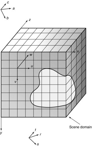
FIGURE 14-1 Drawing provides graphic representation of the four coordinates used in 3D imaging: abc, scanner coordinate system; rst, display coordinate system; uvw, object coordinate system; xyz, scene coordinate system.
The most familiar system is the xyz, the scene or Cartesian coordinate system, as it is commonly called. In this system, the x-, y-, and z-axes are positioned at right angles (orthogonal) to one another. The width of an object is described by the x-axis, whereas the height is described by the y-axis. The z-axis, on the other hand, describes the dimension of depth and adds perspective realism to the image.
Use of the coordinate system allows description of an object by measuring distances from the point of intersection, or zero point. Distances can be positive or negative from the zero point, and images can be manipulated to rotate about the three axes. This rotation occurs in what is referred to as 3D space, and computer software helps the observer to view 3D space by displaying the front, back, top, and bottom of the object, providing a perspective from the observer’s vantage point. The technique is known as computer-aided visualization or 3D visualization, and the application of 3D visualization in medicine is called 3D medical imaging.
In medicine, 3D imaging uses a right-handed x, y, and z coordinate system (Russ, 2006; Udupa and Herman, 2000) because images are displayed on a computer screen. The x, y, and z coordinates define a space in which multidimensional data (a set of slices) are represented. This space is called the 3D space or scene space. The coordinate system helps to define the voxels (volume elements) in 3D space and allows use of the voxel information such as CT numbers or signal intensities in MRI to reconstruct 3D images.
Transforming Three-Dimensional Space
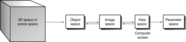
Generally, 3D space can be subjected to a series of common 3D transformations (Fig. 14-2). The radiologic technologist can manipulate scene, structure, geometric, and projective transformations and control image processing and image analysis. The technologist may transform 3D space in four ways (Table 14-2).
TABLE 14-2
Transforming Three-Dimensional Space
| Space Desired | Task Required |
| Image space | Translate, rotate, or scale scenes, objects, or surfaces |
| Object space | Extract structural information about the object from the 3D space |
| Parameter space | Take measurements from the image’s view space on the computer screen |
| View space | View the 2D screen of the computer monitor |
Modeling
The generation of a 3D object using computer software is called modeling. Modeling uses mathematics to describe physical properties of an object. According to one definition, modeling is “a computer simulation of a physical object in which length, width, and depth are real attributes. A model, with x, y, and z axes can be rotated for viewing from different angles” (Microsoft Press, 2002).
Several modeling techniques are used. In extrusion, one of the most common techniques, computer software is used to transform a 2D profile into a 3D object. In Figure 14-3, for example, a square is changed into a box. Extrusion can also generate a wireframe model from a 2D profile. The wireframe is made up of triangles or polygons often referred to as polygonal mesh. Wireframes were common during the early development of 3D display in medicine, and they are still being used today in other applications.
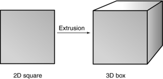
FIGURE 14-3 Extrusion is a modeling technique that generates a 3D object from a 2D profile on a computer screen.
During the next step of modeling, a surface is added to the object by placing a layer of pixels (image mapping) and patterns (procedural textures) on top of the wireframes. The radiologic technologist can control various attributes of the surface, such as its texture.
Shading and Lighting
Shading and lighting also add realism to the 3D object. There are several shading algorithms, including wireframe shading, flat shading, Gouraud shading, and Phong shading. Each technique has its own set of advantages and disadvantages; however, a full discussion of shading algorithms is outside the scope of this chapter. The interested reader should refer to Russ (2006) for detailed descriptions of these algorithms.
Although shading determines the final appearance of surfaces of the 3D object, lighting helps us to see the shape and texture of the object (Fig. 14-4). Various lighting techniques are available to enhance the appearance of the 3D image; one of the most common is called ray tracing, which is described later in this chapter.
Rendering
Rendering is the final step in the process of generating a 3D object. It involves the creation of the simulated 3D image from data collected from the object space. More specifically, rendering is a computer program that converts the anatomical data collected from the patient into the 3D image seen on the computer screen. With most 3D software, the object must be rendered before the effects of lighting and other attributes can be observed. Rendering therefore adds lighting, texture, and color to the final 3D image.
Two types of 3D rendering algorithms are used in radiology: surface rendering and volume rendering. Surface rendering uses only contour data from the set of slices in 3D space, whereas volume rendering makes use of the entire data set in 3D space. Because it uses more information, volume rendering produces a better image than surface rendering, but it takes longer and requires a more powerful computer. Rendering is described subsequently.
CLASSIFICATION OF THREE-DIMENSIONAL IMAGING APPROACHES
Udupa and Herman (2000) have identified three classes of 3D imaging approaches: slice imaging, projective imaging, and volume imaging.
Slice Imaging
Slice imaging is the simplest method of 3D imaging. In 1975 CT operators generated and displayed coronal and sagittal images from the CT axial data set. This technique is known as multiplanar reconstruction (MPR). In the past, other researchers such as Herman and Liu (1977), Marvilla (1978), and Rhodes et al (1980) also used slice imaging to produce coronal, sagittal, and paraxial images from the transaxial scans. Today, MPR is available on all CT and MRI scanners. However, MPR does not produce true 3D images but rather 2D images displayed on a flat computer screen (Dalrymple et al, 2005).
Projective Imaging
Projective imaging is the most popular 3D imaging approach. However, it still does not offer a true 3D mode; it produces a “2.5 D” mode of visualization, an effect somewhere between 2D and 3D. As Udupa and Herman (2000) explain:
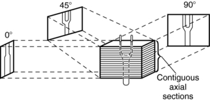
Projective imaging deals with techniques for extracting multidimensional information from the given image data and for depicting such information in the 2D view space by a process of projection. Surface rendering and volume rendering are two major classes of approaches available under projective imaging.
The technique of projection is illustrated in Figure 14-5. The contiguous axial sections represent the volume image data. Information from this volume image data is projected at various angles into the 2D view space.
Volume Imaging
Volume imaging must not be confused with volume rendering. Volume rendering belongs to the class of projective imaging, whereas volume imaging produces a true 3D visualization mode. Volume imaging methods include holography, stereoscopic displays, anaglyphic methods, varifocal mirrors, synthalyzers, and rotating multidiode arrays (Jan, 2005). These methods are beyond the scope of this book.
GENERIC THREE-DIMENSIONAL IMAGING SYSTEM
In a recent article describing the current perspective of 3D imaging, Udupa and Herman (2000) provides a framework for a typical 3D imaging system (Fig. 14-6). Four major elements are noted: input, workstation, output, and the user. Input refers to devices that acquire data. Imaging input devices, for example, would include CT and MRI scanners. The acquired data are sent to the workstation, which is the heart of the system. This powerful computer can handle various 3D imaging operations. These operations include preprocessing, visualization, manipulation, and analysis. Once processing is completed, the results are displayed for viewing and recording onto output devices. Finally, the user can interact with each of the three components—input, workstation, and output—to optimize use of the system.
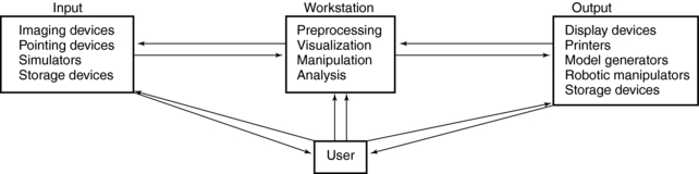
FIGURE 14-6 A typical 3D imaging system consists of four major components: input, workstation, output, and the user.
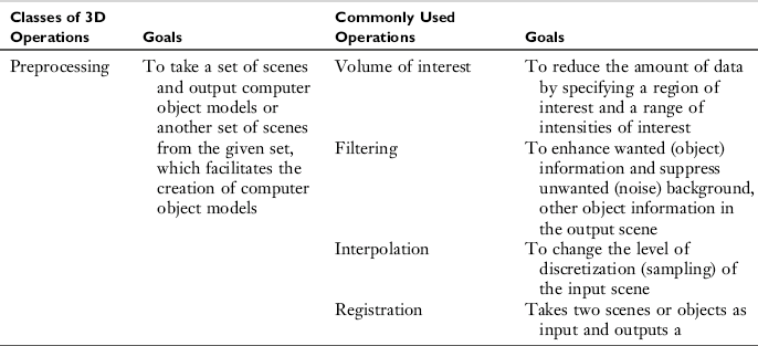
The goals of each of the four major 3D imaging operations and the commonly used processing techniques are summarized in Table 14-3.

TECHNICAL ASPECTS OF THREE-DIMENSIONAL IMAGING IN RADIOLOGY
Definition of Three-Dimensional Medical Imaging
Dr. Gabor Herman of the Medical Image Processing Group at the University of Pennsylvania defines 3D medical imaging as “the process that starts with a stack of sectional slices collected by some medical imaging device and results in computer-synthesized displays that facilitate the visualization of underlying spatial relationships” (Herman, 1993). Additionally, Udupa and Herman (2000) emphasize that the term 3D imaging can also refer to the four categories of 3D operations: preprocessing, visualization, manipulation, and analysis.
Four steps are needed to create 3D images (see Fig. 14-6):
1. Data acquisition. Slices, or sectional images, of the patient’s anatomy are produced. Methods of data acquisition in radiology include CT, MRI, ultrasound, positron emission tomography, single photon emission tomography, and digital radiography and fluoroscopy.
2. Creation of 3D space or scene space. The voxel information from the sectional images is stored in the computer.
3. Processing for 3D image display. This is a function of the workstation and includes the four operations listed previously.
4. 3D image display. The simulated 3D image is displayed on the 2D computer screen.
These four steps vary slightly depending on which imaging modality is used to acquire the data. Each of the four steps is described in detail, using CT as the method of data acquisition.
Data Acquisition
In CT, data are collected from the patient by x-rays and special electronic detectors. Data can be acquired slice by slice with a conventional CT scanner or in a volume with a spiral/helical CT scanner. During slice-by-slice acquisition, the x-ray tube and detectors rotate to collect data from the first slice of the anatomical area of interest; then the data are sent to the computer for image reconstruction. After the first slice is scanned, the tube and detectors stop, the patient is moved into position for the second slice, and scanning continues. The data from the second slice are transferred to the computer for image reconstruction. This “stop-and-go” technique continues until the last slice has been scanned.
One of the fundamental problems of slice-by-slice CT scanning is that certain portions of the anatomy may be missed because motion caused by the patient’s respiration can interfere with scanning or be inconsistent from scan to scan. This problem can lead to inaccurate generation of 3D and multiplanar images. The final 3D image can have the appearance of steplike contours known as the stairstep artifact.
In volume data acquisition, a volume of tissue rather than a slice is scanned during a single breath-hold. This means that more data are sent to the computer for image reconstruction. Volume scanning is achieved because the x-ray tube rotates continuously as the patient moves through the gantry. One advantage of this technique is that more data are available for 3D processing, improving the quality of the resultant 3D image.
Creation of Three-Dimensional Space or Scene Space
All information collected from the voxels that compose each of the scanned slices goes to the computer for image reconstruction. The voxel information is a CT number calculated from tissue attenuation within the voxel. In MRI the voxel information is the signal intensity from the tissue within the voxel. The result of image reconstruction is the creation of 3D space, where all image data are stored (see Fig. 14-7).
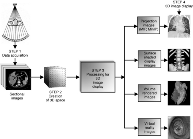
FIGURE 14-7 The major steps in creating 3D images. In Step 1, data are collected from the patient and reconstructed as sectional images, which form 3D space or scene space (Step 2). In Step 3, 3D space can be processed to generate simulated 3D images displayed on a computer screen (Step 4).
Data in 3D space are systematically organized so that each point in 3D space has a specific address. Each point in 3D space represents the information (CT number or MRI signal intensity) of the voxels within the slice.
Processing for Three-Dimensional Image Display
Processing, which is a major step in the creation of simulated 3D images for display on a 2D computer screen, is accomplished on the workstation. Although it is not within the scope of this chapter to address these operations in detail, it is important that technologists have an understanding of how sectional images are transformed into 3D images as illustrated in Figure 14-7.
In 1990, Mankovich et al (1990) identified two classes of processing to explain 3D image display: voxel-based processing and object-based processing. Voxel-based processing “makes determinations about each voxel and decides to what degree each should contribute to the final 3D display,” whereas object-based processing “uses voxel information to transform the images into a collection of objects with subsequent processing concentrating on the display of the objects.”
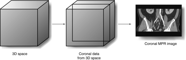
Voxel-based processing was used as early as 1975 as a means of generating coronal, sagittal, and oblique images from the stack of contiguous transverse axial set of images—the technique of MPR. Although MPR is not a true 3D display technique, it does provide additional information to enhance our understanding of 3D anatomy (Beigleman-Aubry et al, 2005; Lell et al, 2006). In MPR, the computer scans the 3D space and locates all voxels in a particular plane to produce that particular image (Fig. 14-8).
Object-based processing involves several processing methods to produce a model (called an object model or object representation) from the 3D space and transforms it into a 3D image displayed on a computer screen. According to Russ (2006) and others (Dalrymple et al, 2005; Lell et al, 2006; Udupa and Herman, 2000), the processing of an object model into a simulated 3D image involves steps such as the following:
1. Segmentation is a processing technique used to identify the structure of interest in a given scene. It determines which voxels are a part of the object and should be displayed and which are not and should be discarded. Thresholding is a method of classifying the types of tissues, such as, say bone, soft tissue, or fat, represented by each of the voxels. The CT number is used for assigning thresholds to tissues.
2. Object delineation is portraying an object by drawing it. It involves boundary and volume extraction and detection methods. Although boundary extraction methods search the 3D space for only those voxels that define the outer or inner border or surface of the object called the object contour, volume extraction methods find all the voxels in 3D space and its surface.
3. Rendering is the stage when an image in 3D space is transformed into a simulated 3D image to be displayed on a 2D computer monitor. Rendering is a computer display technology-based approach (computer program) and therefore requires specific hardware and software to deal with millions of points identified in 3D space.
RENDERING TECHNIQUES
Two classes of rendering techniques are common in radiology: surface rendering and volume rendering (Beigleman-Aubry et al, 2005; Dalrymple et al, 2005; Fishman et al, 2006; Kalender, 2005; Lell et al, 2006; Pickhardt, 2004; Silva et al, 2006; Udupa and Herman, 2000).
Surface Rendering
Surface rendering, or shaded surface display (SSD), has evolved through the years with significant improvements in image quality (Fig. 14-9). In surface rendering, the computer creates “an internal representation of surfaces that will be visible in the displayed image. It then ‘lights’ them according to a standard protocol, and displays an image according to its calculation of how the light rays
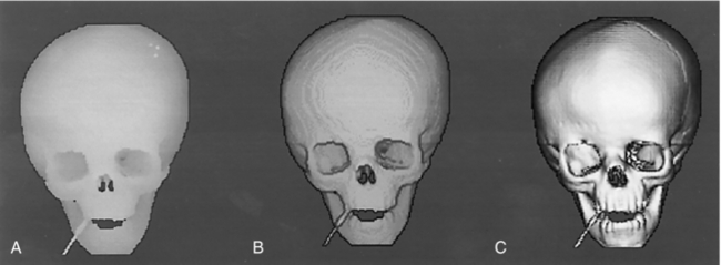
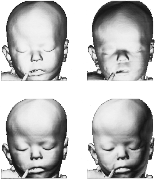
FIGURE 14-9 The evolution of surface rendering technique, demonstrating the improvement in image quality. A, Older processing methods. B, Recent methods. C, Current techniques.
1. Scan the 3D space or scene space for all voxel information relating to the object to be displayed.
2. Create the surface of the object by using contour information (segmentation) obtained by thresholding. The threshold setting determines whether skin or bone surfaces will be displayed. The 3D images of the skull shown in Figure 14-9 are examples of surface rendering.
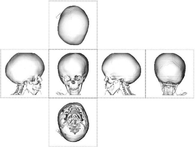
3. Select the viewing orientation to be processed for 3D image display and assign the position of one or more lighting sources. A standard set of views is shown in Figure 14-10.
4. Surface rendering begins. The pixels of the object to be displayed are shaded for photorealism and particularly to give the illusion of depth. Those pixels farthest away from the viewer are darker than those closer to the viewer.
would be reflected to the viewer’s eye” (Schwartz, 1994).
According to Udupa and Herman (2000), surface rendering involves essentially two steps: surface formation and depiction on a computer screen (rendering) (see box above). Surface formation involves the operation of contouring. Rendering follows surface formation and is intended to add photorealism and create the illusion of depth in an image, making it appear 3D on a 2D computer screen. A simulated light source can be positioned at different locations to enhance features of the displayed 3D image (see Fig. 14-4).
The advantage of surface rendering techniques is that they do not require a lot of computing power because they do not use all the voxel information in 3D space to create the 3D image. Only contour information is used. However, this results in poor image information content.
Heath et al (1995) demonstrated this disadvantage when they used surface rendering to image the liver. They reported the following:
No information about structures inside or behind the surface such as vessels within the liver capsule or thrombus within a vessel is displayed. In medical volume data, which are affected by volume averaging because of finite voxel size, clear-cut edges and surfaces are often difficult or impossible to define. Many voxels necessarily contain multiple tissue types and classifying them as being totally not part of a given tissue introduces artifacts into the image. Surface renderings are very sensitive to changes in threshold, and it is often difficult to determine which threshold yields the most accurate depiction of the actual anatomic structures.
Figure 14-11 illustrates surface rendering numerically. Numbers represent the voxel values for a sample 2D data set. An algorithm is applied to locate a “surface” within the data set at the margin of the region of voxels with intensities ranging from 6 to 9. Standard computer graphics techniques are then used to generate a surface that represents the defined region of voxel values (Heath et al, 1995).

Volume Rendering
Volume rendering is a more sophisticated technique and produces 3D images that have a better image quality and provide more information compared with surface rendering techniques (Neri et al, 2007). Volume rendering overcomes several of the limitations of surface rendering because it uses the entire data set from 3D space. Because of this, volume rendering requires more computing power and is more expensive than surface rendering.
Udupa and Herman (2000) describe the conceptual framework of volume rendering:
The scene is considered to represent blocks of translucent colored jelly whose color and opacity (degree of transparency) are different for different tissue regions. The goal of rendering is to compute images that depict the appearance of this block from various angles, simulating the transmission of light through the block as well as its reflection at tissue interfaces through careful selection of color and opacity.
The two stages to volume rendering are preprocessing the volume and rendering.
Preprocessing: Preprocessing involves several image processing operations, including segmentation, also referred to as classification, to determine the tissue types contained in each voxel and to assign different brightness levels or color. In addition, a partial transparency (0% to 100%) is also assigned to different tissues that make up 3D space. Three tissue types—fat, soft tissue, and bone—are used for voxel classification.
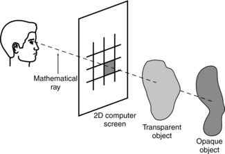
Rendering: Rendering is stage two of the volume-rendering technique. It involves image projection to form the simulated 3D image. One popular method of image projection is ray tracing, illustrated in Figure 14-12. During ray tracing, a mathematical ray is sent from the observer’s eye through the 2D computer screen to pass through the 3D volume that contains opaque and transparent objects. The pixel intensity on the screen for that single ray is the average of the intensities of all the voxels through which the ray travels. As Mankovich et al (1990) explain, “If all objects are opaque, only the nearest object is considered, and the ray is then traced back to the light source for calculation of the reflected intensity. If the nearest object is transparent, the ray is diminished and possibly refracted to the next nearest object and so on until the light is traced back to the source.”
Unlike surface rendering, volume rendering offers the advantage of seeing through surfaces, allowing the viewer to examine both external and internal structures (Fig. 14-13). A numerical illustration of how this is accomplished is shown in Figure 14-14. Opacities of 0% and 100% are assigned for values of 5 or lower and 9 or higher, respectively. The resulting intermediate opacities for values 6, 7, and 8 are 25%, 50%, and 75%, respectively. The lower portion of the diagram shows the equation and progressive computational results used to determine weighted summation along the “ray” through the volume. The resulting displayed value (6) is affected by both opacity (as determined in the graph at the top) and the value of underlying voxels (Calhoun et al, 1999).
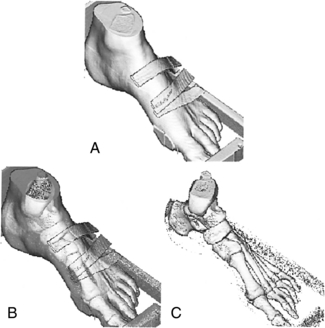
FIGURE 14-13 A, A surface-rendered image. B, An example of volume rendering, in which the soft tissues have been made transparent; it allows the viewer to see both the skin and bone surfaces at the same time. C, The entire surface is removed.
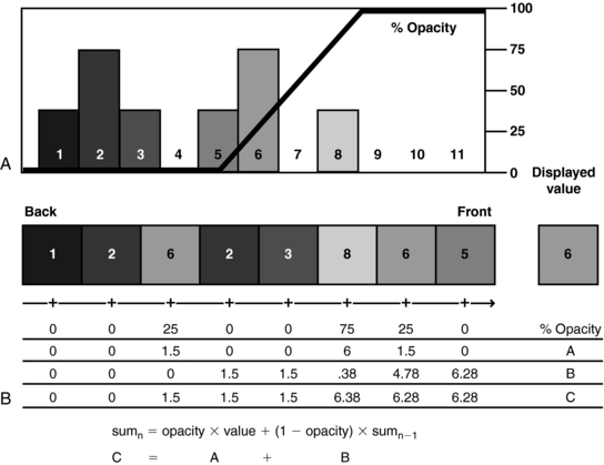
FIGURE 14-14 Diagram illustrates volume-rendering technique. A histogram of the voxel values (A) in the data “ray” (B).
The effect of SSD and volume-rendering techniques on image details is clearly illustrated in Figure 14-15.
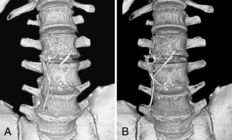
FIGURE 14-15 SSD and volume-rendered images of an inferior vena cava filter overlying the spine. A, SSD creates an effective 3D model for looking at osseous structures in a more anatomical perspective than is achieved with axial images alone. It was used in this case to evaluate pelvic fractures not included on this image. B, Volume rendering achieves a similar 3D appearance to allow inspection of the bone surfaces in a relatively natural anatomical perspective. In addition, the color assignment tissue classification possible with volume rendering allows improved differentiation of the inferior vena cava filter from the adjacent spine. From Dalrymple NC et al: Introduction to the language of three-dimensional imaging with multidetector CT, Radiographics 25:1409-1428, 2005. Figure and legend reproduced by permission of the Radiological Society of North America and the authors.
Intensity Projection Renderings
As noted in Figure 14-8, processing of image data from 3D space can also generate intensity projection images. These images, as Kalender (2005) points out, are “an extension of MPR techniques and consists of generating arbitrary thick slices (slabs) from thin slices reducing the noise level and possibly also improving the visualization of structures, for example, vessels present in the several thin slices … . The term sliding thin slabs is known for this technique … .” In addition, Dalrymple et al (2005) note that “multiplanar images can be ‘thickened’ into slabs by tracing a projected ray through the image to the viewer’s eye, then processing the data encountered as the ray passes through the stack of reconstructed sections along the line of sight according to one of several algorithms.” This is clearly illustrated in Figure 14-16.
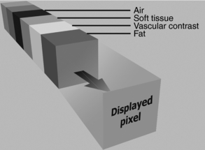
FIGURE 14-16 Row of data encountered along a ray of projection. The data consist of attenuation information calculated in Hounsfield units. The value of the displayed 2D pixel is determined by the amount of data included in the calculation (slab thickness) and the processing algorithm (MIP, MiniIP, or AIP or ray sum). From Dalrymple NC et al: Introduction to the language of three-dimensional imaging with multidetector CT, Radiographics 25:1409-1428, 2005. Figure and legend reproduced by permission of the Radiological Society of North America and the authors.
The algorithms for sliding thin slabs (STS) (or thickening of MPR images) include average intensity projection (AIP), maximum intensity projection (MIP), and minimum intensity projection (MinIP).
Average Intensity Projection: The AIP technique is an algorithm that is intended to create a thick MPR image by using the average of the attenuation through the tissues of interest to calculate the pixel viewed on the computer, as is clearly illustrated in Figure 14-17. The effects of the AIP algorithm on an image are shown in Figure 14-18.
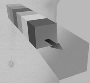
FIGURE 14-17 AIP of data encountered by a ray traced through the object of interest to the viewer. The included data contain attenuation information ranging from that of air (black) to that of contrast media and bone (white). AIP uses the mean attenuation of the data to calculate the projected value. From Dalrymple NC et al: Introduction to the language of three-dimensional imaging with multidetector CT, Radiographics 25:1409-1428, 2005. Figure and legend reproduced by permission of the Radiological Society of North America and the authors.
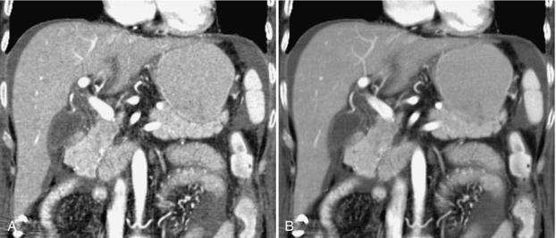
FIGURE 14-18 Effects of AIP on an image of the liver. A, Coronal reformatted image created with a default thickness of 1 pixel (approximately 0.8 mm). B, Increasing the slab thickness to 4 mm by using AIP results in a smoother image with less noise and improved contrast resolution. The image quality is similar to that used in axial evaluation of the abdomen. From Dalrymple NC et al: Introduction to the language of three-dimensional imaging with multidetector CT, Radiographics 25:1409-1428, 2005. Figure and legend reproduced by permission of the Radiological Society of North America and the authors.
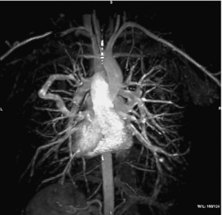
Maximum Intensity Projection: MIP is a volume-rendering 3D technique that originated in magnetic resonance angiography (MRA) and is now used frequently in CTA. In MIP, the algorithm is such that only the tissues with the greatest attenuation will be displayed for viewing by an observer, as is illustrated in Figure 14-19.
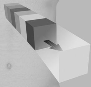
FIGURE 14-19 MIP of data encountered by a ray traced through the object of interest to the viewer. The included data contain attenuation information ranging from that of air (black) to that of contrast media and bone (white). MIP projects only the highest value encountered. From Dalrymple NC et al: Introduction to the language of three-dimensional imaging with multidetector CT, Radiographics 25:1409-1428, 2005. Figure and legend reproduced by permission of the Radiological Society of North America and the authors.
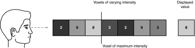
MIP does not require sophisticated computer hardware because, like surface rendering, it makes use of less than 10% of the data in 3D space. Figure 14-20 details the underlying concept of MIP. Essentially, the MIP computer program renders a 2D image on a computer screen from a 3D data set (slices) as follows:
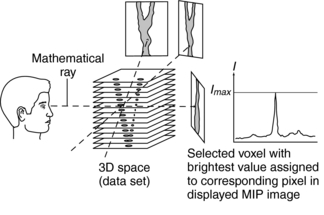
1. A mathematical ray (similar to the one in ray tracing) is projected from the viewer’s eye through the 3D space (data set).
2. This ray passes through a set of voxels in its path.
3. The MIP program allows only the voxel with the maximum intensity (brightest value) to be selected.
4. The selected voxel intensity is then assigned to the corresponding pixel in the displayed MIP image.
5. The MIP image is displayed for viewing (Fig. 14-21).
A numerical illustration the MIP technique is clearly shown in Figure 14-22.
MIP images can also be displayed in rapid sequence to allow the observer to view an image that can be rotated continuously back and forth to enhance 3D visualization of complex structures with postprocessing techniques. Figure 14-23 shows multiple projections that vary only slightly in degree increments.
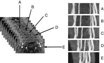
FIGURE 14-23 A complete projection image at different viewing angles. Postprocessing of the 3D data set can generate different views to allow the observers to rotate the image back and forth to enhance the perception of 3D relationships in the vessels. From Laub G et al: Magnetic resonance angiography techniques, Electromedica 66:68-75, 1998.
In the past, one of the basic problems with the MIP technique is that “images are three-dimensionally ambiguous unless depth cues are provided” (Heath et al, 1995). To solve this problem, a depth-weighted MIP can be used to deal with the intensity of the brightest voxel, depending on its distance from the viewer. Other limitations include the inability of the MIP program to show superimposed structures because only one voxel (the one with the maximum intensity) in the set of voxels traversed by a ray is used in the MIP image display. Additionally, MIP generates a “string of beads” artifact because of volume averaging problems with tissues that have lower intensity values (Heath et al, 1995) and artifacts arising from pulsating vessels and respiratory motion.
A significant advantage of the MIP algorithm is that it has become the most popular rendering technique in CTA (Dalrymple et al, 2005; Fishman et al, 2006; Lell et al, 2006) and MRA (Dalrymple et al, 2005) because vessels containing contrast medium are clearly seen. Additionally, because MIP uses less than 10% of the volume data in 3D space, it takes less time to produce 3D simulated images than do volume-rendering algorithms.
Minimum Intensity Projection: The MinIP algorithm ensures that only the tissues with the minimum or lowest attenuation will be displayed for viewing by an observer. This is illustrated in Figure 14-24. Of the three intensity projection techniques, the MinIP is the least used; however, MinIP images may be useful in providing a “valuable perspective in defining lesions for surgical planning or detecting subtle small airway diseases” (Dalrymple et al, 2005).
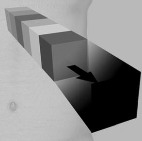
FIGURE 14-24 MinIP of data encountered by a ray traced through the object of interest to the viewer. The included data contain attenuation information ranging from that of air (black) to that of contrast media and bone (white). MinIP projects only the lowest value encountered. From Dalrymple NC et al: Introduction to the language of three-dimensional imaging with multidetector CT, Radiographics 25:1409-1428, 2005. Figure and legend reproduced by permission of the Radiological Society of North America and the authors.
Virtual CT Endoscopy
The CT image data from 3D space can be processed in such a way by using sophisticated computer algorithms to generate what has been referred to as virtual endoscopic images. These images are based on both 2D and 3D CT image data sets by using a technique known as perspective volume rendering (pVR) (Kalender, 2005). pVR is used to examine hollow structures such as the colon (CT colonoscopy) and the bronchi (CT bronchoscopy), for example. Furthermore, pVR can create an approach that allows the operator to “fly-through” the hollow structure. Virtual CT endoscopy is described in detail in Chapter 15.
Comparison of Three-Dimensional Rendering Techniques
One early comprehensive comparison of surface and volume rendering techniques was performed in 1991 by Udupa and Herman. They concluded that the surface method had a minor advantage over the volume methods with respect to display ability, clarity of the display, smoothness of ridges and silhouettes, computational time, and storage requirements. It had a significant advantage with its time and storage requirements.
Later in 1995, Heath et al (1995) compared surface rendering, volume rendering, and MIP with spiral/helical CT during arterial portography. They compared the techniques with respect to seven parameters: depiction of 3D relationships, edge delineation, demonstration of overlapping structures, depiction of vessel lumen, percentage of data used, artifacts, and computational cost. Their results are summarized in Table 14-4. It is clearly apparent that volume rendering is superior in all parameters compared; however, it has the highest computational cost.
TABLE 14-4
Comparison of Three-Dimensional Rendering Techniques in Medical Imaging
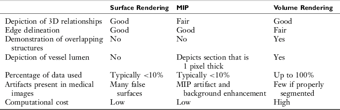
From Heath DG et al: Three-dimensional spiral CT during arterial portography: comparison of three rendering techniques, Radiographics 15:1001-1011, 1995.
One of the characteristic features of the MIP technique is that it removes discarded data having low values. The SSD technique removes all data with the exception of the data that are associated with the surface and, as mentioned in Table 14-4, typically uses less than 10% of the data. The effect of this data limitation is illustrated in Figure 14-25.

FIGURE 14-25 Data limitations of SSD. Surface data are segmented from other data by means of manual selection or an attenuation threshold. The graph in the lower part of the figure represents an attenuation threshold selected to include the brightly contrast-enhanced renal cortex and renal vessels during CTA. The “virtual spotlight” in the upper left corner represents the gray-scale shading process, which in reality is derived by means of a series of calculations. To illustrate the “hollow” data set that results from discarding all but the surface rendering data, the illustration was actually created by using a volume-rendered image of the kidney with a cut plane transecting the renal parenchyma. Subsequent editing was required to remove the internal features of the object while preserving the surface features of the original image. HU, Hounsfield units. From Dalrymple NC et al: Introduction to the language of three-dimensional imaging with multidetector CT, Radiographics 25:1409-1428, 2005. Figure and legend reproduced by permission of the Radiological Society of North America and the authors.
Although volume-rendered images may look similar to images generated by the SSD technique, the use of 100% of the acquired data set and “assigning a full spectrum of opacity values and separation of the tissue classification and shading processes provide a much more robust and versatile data set than the binary system offered by SSD” (Dalrymple et al, 2005). This is clearly shown in Figure 14-26.
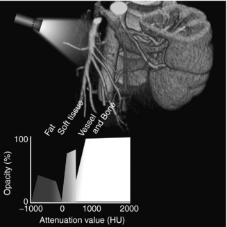
FIGURE 14-26 Data-rich nature of volume rendering. The graph in the lower part of the figure shows how attenuation data are used to assign values to a histogram-based tissue classification consisting of deformable regions for each type of tissue included. In this case, only fat, soft tissue, vessels, and bone are assigned values, but additional classifications can be added as needed. Opacity and color assignment may vary within a given region, and the shape of the region can be manipulated to achieve different image effects. Because there is often overlap in attenuation values between different tissues, the classification regions may overlap. Thus, accurate tissue and border classification may require additional mathematical calculations that take into consideration the characteristics of neighboring data. HU, Hounsfield units. From Dalrymple NC et al: Introduction to the language of three-dimensional imaging with multidetector CT, Radiographics 25:1409-1428, 2005. Figure and legend reproduced by permission of the Radiological Society of North America and the authors.
In the past years, 3D volume rendering has been shown to be useful in a wide range of clinical applications (Calhoun et al, 1999), including the thoracic aorta (Christine et al, 1999) and in evaluating carotid artery stenosis (Leclerc et al, 1999).
More recent discussions of the use of 3D rendering techniques for clinical imaging using the data obtained from Multislice CT scanners have been reported by several authors, including Kalender, 2005; Dalrymple et al, 2005; Silva et al, 2006; Lell et al, 2006; and Fishman et al, 2006, and the interested student should refer to these original reports for more information.
Some important considerations to note, however, when these 3D imaging techniques are used are noted by several authors as follows:
• “Appreciation of the strengths and weaknesses of rendering techniques is essential to appropriate clinical application and is likely to become increasingly important as networked 3D capability can be used to integrate real-time rendering into routine image interpretation.” (Dalrymple et al, 2005)
• “My own expectation is that volume rendering with user friendly, preset evaluation protocols and intelligent editing tools will prevail as the method of choice in 3D display forms. However, they will only supplant and augment, but not replace 2D displays.” (Kalender, 2005)
• “Generating ‘boneless’ 3D images became possible with modern postprocessing techniques, but one should keep in mind the potential pitfalls of these techniques and always double- check the final results with source or MPR images.” (Lell et al, 2006)
• “Although different systems have unique capabilities and functionality, all provide the options of volume rendering and maximum intensity projection for image display and analysis. These two post processing techniques have different advantages and disadvantages when used in clinical practice, and it is important that radiologists understand when and how each technique should be used.” (Fishman et al, 2006)
• “To avoid potential pitfalls in image interpretation, the radiologist must be familiar with the unique appearance of the normal anatomy and of various pathologic findings when using virtual dissection with two-dimensional axial and 3D endoluminal CT colonographic image data sets.” (Silva et al, 2006)
EDITING THE VOLUME DATA SET
The purpose of editing the volume data set is intended for clarity of 3D image display. This is well described by Fishman et al (2006), and the interested reader should refer to the article for a detailed account of the procedure. In summary, Fishman et al (2006) note the following:
1. The volume-rendered 3D technique is much better than the MIP technique for a clear display of the anatomy of interest in the volume data set. The MIP cannot display the 3D anatomical relationships, only because it is 2D.
2. For better clarity of anatomical details, the volume data set must be edited by using thinner slabs compared with the entire volume data set.
3. Several editing tools are available to change the appearance of the images. These include windowing (window width and window length manipulation), color and shading tools, and tools that allow the operator to change the opacity or the transparency of the image display (Fishman et al, 2006) and segmentation (Dalrymple, 2005; Lell et al, 2006).
EQUIPMENT
Equipment for 3D image processing falls into two categories: the CT or MRI scanner console and stand-alone computer workstations. Both types of equipment use software designed to perform several image processing operations, such as interactive visualization, multi-image display, analysis and measurement, intensity projection renderings, and 3D rendering. Most postprocessing for 3D imaging is done on stand-alone dedicated workstations that are becoming more popular as their costs decrease.
Stand-Alone Workstations
A number of popular CT equipment manufacturers provide 3D packages for their CT and MRI scanners, and many are offering both 3D hardware and software packages for use in radiology. Although the technical specifications of each workstation vary depending on the manufacturer, typical 3D processing techniques include software to perform the following:
• Surface and volume rendering
• Slice plane mapping. This technique allows two tissue types to be viewed at the same time.
• Slice cube cuts. This is a processing technique that allows the operator to slice through any plane to demonstrate internal anatomy.
• Transparency visualization. This processing technique allows the operator to view both surface and internal structures at the same time.
• Four-dimensional angiography. This technique shows bone, soft tissue, and blood vessels at the same time and allows the viewer to see tortuous vessels with respect to bone.
• Disarticulation. This SSD technique allows the viewer to enhance the visualization of certain structures by removing others.
• Virtual reality imaging. Some workstations are also capable of virtual endoscopy, a processing technique that allows the viewer to look into the lumen of the bronchus and colon, for example. It is also possible for the viewer to “fly through” the 3D data set. Virtual CT endoscopy is described in Chapter 15.
CLINICAL APPLICATIONS OF THREE-DIMENSIONAL IMAGING
One of the major motivating factors for the development and application of 3D imaging in medicine is to improve the communication gap between the radiologist and the surgeon. 3D imaging can help radiologists locate the condition and identify the best way to demonstrate it. Interestingly, craniofacial surgery was one of the first clinical applications of 3D medical imaging. Today, 3D medical imaging is used for applications ranging from orthopedics to radiation therapy (Calhoun et al, 1999; Dalrymple et al, 2005; Fishman et al, 1992; Fishman et al, 2006; Kalender, 2005; Lell et al, 2006; Silva et al, 2006; Udupa and Herman, 1991; Zonneveld and Fukuta, 1994).
The applications of 3D imaging in CT, MRI, nuclear medicine, and ultrasonography continue to evolve at a rapid rate, with most of the work being done in CT and MRI. For example, 3D imaging has provided the basis for endoscopic imaging, where the viewer can “fly through” CT and MRI data sets with the goal of performing “virtual endoscopy.” The most recent clinical application of 3D imaging is virtual dissection, “an innovative technique whereby the three-dimensional (3D) model of the colon is virtually unrolled, sliced open, and displayed as a flat 3D rendering of the mucosal surface, similar to a gross pathologic specimen” (Silva et al, 2006).
To date, clinical applications of 3D imaging in CT have been in the craniomaxillofacial complex, musculoskeletal system, central nervous system, cardiovascular system, pulmonary system, gastrointestinal system, and genitourinary system and in radiation treatment planning for therapy. In the craniomaxillofacial complex, for example, 3D imaging has been used to evaluate congenital and developmental deformities (shape of the deformed skull and the extent of suture ossification) and to assess trauma (bone fragment displacement and fractures).
3D imaging can demonstrate complex musculoskeletal anatomy and is used to study acetabular and calcaneal trauma, muscle atrophy, spinal conditions, and trauma of the spine, knee, carpal bones, and shoulder.
The development of CTA opened up additional avenues for the use of 3D imaging in the evaluation of cerebral aneurysms and arteriovenous malformations. It has been applied in CT of the gastrointestinal system, primarily imaging the liver, and genitourinary systems, primarily in kidney and bladder assessment. 3D volume rendering provides accurate evaluation of the thoracic aorta and internal carotid artery stenosis.
In radiation therapy, 3D imaging is especially used to superimpose isodose curves on sectional anatomy for the purpose of providing a clear picture of tissues and organs that receive various degrees of radiation dose. This is essential to demonstrate that the tumor receives maximum dose with minimum dose to the surrounding healthy tissues.
The student should refer to the reports by Dalrymple et al, 2005; Silva et al, 2006; Lell et al, 2006; Fatterpekar et al, 2006; Beigleman-Aubry et al, 2005; Fayad et al, 2005; Lawler et al, 2005; Pickhardt, 2004, and Fishman et al, 2006, for more recent applications of 3D imaging in clinical practice.
FUTURE OF THREE-DIMENSIONAL IMAGING
The first two decades of 3D imaging have generated a new and vast knowledge base on the technology of 3D imaging and on its clinical role in medicine. It has provided additional information that has helped in the diagnostic interpretation of images and enhanced communication between radiologists and surgeons and other physicians.
As research and development in 3D imaging continue, experts predict promising gains for radiology. Additionally, developments can be expected in computer architecture that will boost processing power and speed. Software developments will include improvements in segmentation techniques, for example. Also the cost of dedicated computer hardware and software will decrease, and personal computer–based workstations will become available. 3D rendering is now possible on the Internet.
As the technology for 3D imaging becomes increasingly sophisticated and better refined, clinical applications will expand and 3D imaging will be applied to other areas of the body. Applications in CT, MRI, and other imaging modalities will expand with the goal of providing additional information to support and validate diagnostic interpretation.
3D imaging involves digital image postprocessing techniques. The series of articles by Barnes (2006) entitled “Medical Image Processing has Room to Grow” point out that this is an area of active research, and there will be increasingly new applications for use in medicine, particularly in medical imaging.
ROLE OF THE RADIOLOGIC TECHNOLOGIST
As 3D imaging technology expands and becomes commonplace in medical imaging and radiation therapy, it is likely that radiologic technologists will play an increasing role in image processing and analysis techniques. Radiologic technologists may need to expand their knowledge base to include a basic understanding of 3D imaging concepts. Educational programs in the radiologic technology may need to offer courses that prepare students to perform 3D imaging and various image postprocessing for digital images in medical imaging.
To perform quality 3D medical imaging, the technologist and the radiologist must work as a team. Technical ability in performing CT or MRI examinations and an understanding of the 3D imaging process and other postprocessing digital techniques are equally important. In addition, effective communication between the technologist and radiologist is vital in performing 3D medical imaging and will become even more important as the technology expands to provide new clinical applications.
REFERENCES
Barnes E: Medical image processing has room to grow: parts 1, 2, and 3 (2006): AuntMinni.com. Accessed December 2006.
Beigelman-Aubry, C, et al. Multi-detector row CT and postprocessing techniques in the assessment of diffuse lung disease. Radiographics. 2005;25:1639–1652.
Calhoun, PS, et al. Three-dimensional volume rendering of spiral CT data: theory and method. Radiographics. 1999;19:745–764.
Dalrymple, NC, et al. Introduction to the language of three-dimensional imaging with multidetector CT. Radiographics. 2005;25:1409–1428.
Fayad, LM, et al. Multidetector CT of the musculoskeletal disease in the pediatric patient: principles, techniques, and clinical applications. Radiographics. 2005;25:603–618.
Fishman, EK, et al. Volume rendering versus maximum intensity projection in CT angiography: what works best, when, and why. Radiographics. 2006;26:905–922.
Heath, DG, et al. Three-dimensional spiral CT during arterial portography: comparison of three rendering techniques. Radiographics. 1995;15:1001–1011.
Herman, GT, Liu, HK. Display of three-dimensional information in computed tomography. J Comput Assist Tomogr. 1977;1:155–160.
Herman, GT. 3D display: a survey from theory to applications. Comput Med Imag Graph. 1993;17:131–142.
Hoffman, H, et al. Paleoradiology: advanced CT in the evaluation of Egyptian mummies. Radiographics. 2002;22:377–385.
Jan, J. Medical image processing, reconstruction and restoration (signal processing and communications). Boca Raton: CRC Press, 2005.
Kalender W: Computed tomography: fundamentals, system technology, image quality, applications, Munich, Germany, 2005, Publicis.
Lawler, LP, et al. Adult uteropelvic junction obstruction: insights with three-dimensional multi-detector row CT. Radiographics. 2005;25:121–134.
Leclerc, X, et al. Internal carotid artery stenosis: CT angiography with volume rendering. Radiology. 1999;210:673–682.
Lell, MM, et al. New techniques in CT angiography. Radiographics. 2006;26:S45–S62.
Macari, M, Bini, EJ. CT colonography: where have we been and where are we going? Radiology. 2005;237:819–833.
Mahoney, DP. The art and science of medical visualization. Comput Graph World. 1996;14:25–32.
Mankovich, NJ, et al. Three-dimensional image display in medicine. J Digit Imaging. 1990;3:69–80.
Marvilla, KR. Computer reconstructed sagittal and coronal computed tomography head scans: clinical applications. J Comput Assist Tomogr. 1978;2:120–123.
Microsoft Press. Computer dictionary, 5. Redmond, Wash: Microsoft Press, 2002.
Neri E, et al, eds. Image processing in radiology. New York: Springer, 2007.
Pickhardt, PJ. Differential diagnosis of polypoid lesions seen at CT colonoscopy (virtual colonoscopy). Radiographics. 2004;24:1535–1559.
Rhodes, ML, et al. Extracting oblique planes from serial CT sections. J Comput Assist Tomogr. 1980;4:649–657.
Rubin, GD, et al. Perspective volume rendering of CT and MR images: applications for endoscopic imaging. Radiology. 1996;199:321–330.
Russ, JC. The image processing handbook, 5. Boca Raton: CRC Press, 2006.
Schwartz, B. 3D computerized medical imaging. Med Device Res Rep. 1994;1:8–10.
Silva, AC, et al. Three-dimensional virtual dissection at CT colonography: unraveling the colon to search for lesions. Radiographics. 2006;26:1669–1686.
Udupa, JK. Three-dimensional visualization and analysis methodologies: a current perspective. Radiographics. 1999;19:783–803.
Udupa J, Herman G: 3D imaging in medicine, Boca Raton, 1991, CRC Press.
Udupa JK, Herman GT, eds. 3D imaging in medicine, 2, Boca Raton, Fla: CRC Press, 2000.
Vining, DJ. Virtual endoscopy flies viewer through the body. Diagn Imaging. 1996;3:127–129.
Wu, CM, et al. Spiral CT of the thoracic aorta with 3D volume rendering: a pictorial review. Cardiaovasc Intervent Radiol. 1999;22:159–167.
Yasuda, T, et al. 3D visualization of an ancient Egyptian mummy. IEEE Comput Graphics Appl. 1992;2:13–17.
Zonneveld, FW, Fukuta, K. A decade of clinical three-dimensional imaging: a review, 2: clinical applications. Invest Radiol. 1994;29:574–589.