Chapter Seven Single case (n = 1) designs
Introduction
We have discussed research designs involving the comparison of groups of participants selected from a population. These designs provide evidence concerning the general causes of diseases, or the overall effectiveness of interventions. However, health professionals often work with individual patients and need to understand the specific causes of their problems and the effectiveness of treatments as applied to them as individuals. n = 1 designs illustrate the close relationship between the principles for conducting research and everyday clinical practice.
The aim of the present chapter is to examine single subject (n = 1) designs, as applied by a variety of health professionals in natural clinical settings. You will be able to recognize close similarities between these designs and the quasi-experimental designs discussed in the previous chapter.
AB designs
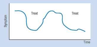
Let us consider a simple example to illustrate the basic procedures involved in using n = 1 designs. Imagine that a patient is admitted to your ward suffering from a condition that involves having a high temperature. Before an appropriate intervention is devised, the patient’s temperature is recorded every 15 minutes, for 2 hours. Following this time interval, the patient is given medication to reduce temperature. The question here is: ‘How do we show that the medication was effective for reducing the patient’s temperature?’ Obviously, we need to show that the patient’s temperature had fallen following the administration of the medication. Figure 7.1 illustrates a possible outcome.
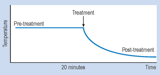
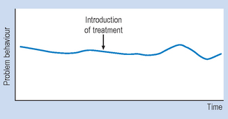
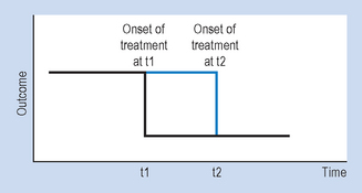
Let us assume that the drug is known to act quickly, say in 20 minutes. The evidence shown in Figure 7.1 would be clearly consistent with the hypothesis that the medication caused a decrease in the patient’s temperature. Let us generalize this example to n = 1 designs used in various settings. Figure 7.2 illustrates the general conventions used in n = 1 designs.
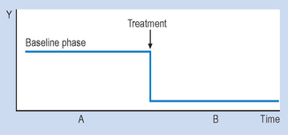
Therefore, an AB design involves taking observations during phase A, introducing an appropriate intervention, and then taking observations during B. It might have occurred to you that several of the threats to validity can be identified in AB designs. An obvious threat to validity is maturation, that is, recovery or deterioration occurring in the patient that might influence the readings on the outcome variable. Another possible threat is history, that is, influences on the patient other than the actual intervention. In the example we just looked at, one could also argue that perhaps the patient’s temperature would have gone down even without the drug, because of the condition improving by itself or the environment of the ward (maturation), or perhaps the ward was air-conditioned and the patient would have cooled down anyway, drugs or not (history).
Next, we look at ABAB designs, which provide stronger control for extraneous variables than AB designs.
ABAB designs
The basic feature of ABAB designs is the alternation of intervention with no-intervention or baseline phases. That is, the researcher introduces the intervention following a baseline or no-intervention phase, then the intervention is withdrawn and then later re-introduced. Observations are recorded during each phase and this approach permits control for the previously discussed threats to validity.
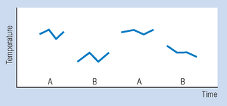
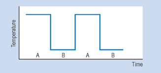
Figure 7.3 illustrates the outcomes for a hypothetical drug study using an ABAB design. When the drug is withdrawn (second A) the patient’s temperature returns to previous levels. When the drug is re-introduced (second B), the patient’s temperature declines. Clearly, such an outcome is consistent with a causal relationship between the independent variable (intervention) and the outcome or dependent variable (observations of temperature). Figure 7.4 demonstrates the idealized results expected using ABAB designs with a highly effective rapid-onset intervention.
Although the above design is useful for demonstrating causal effects in a single individual, there are situations where it is inappropriate. ABAB designs are not particularly useful when there is a good reason to expect that the effects for an intervention are known to be irreversible following the intervention. For example, if the medication used in the previous example involved antibiotics, then the discontinuation of such drugs after a period might not result in the re-emergence of the symptoms since the antibiotics might well cure the underlying problem. Even when reversal is possible, it might not be ethical. Clearly, if we have succeeded in establishing desirable effects in our client during the first B period, we might well be reluctant to reverse this for the sake of demonstrating causal relationships.
Multiple baseline designs
Multiple baseline designs involve the use of concurrent observations to generate two or more baselines. Given two or more baselines, the investigator has the opportunity to introduce intervention affecting only one set of observations, while using the other(s) as a control. We will examine a hypothetical clinical problem to illustrate these designs.
Imagine that we have a brain-damaged client showing aggressive behaviours that disrupt therapy. Therapy is offered in two situations, say occupational therapy (Situation 1) and speech therapy (Situation 2). A behavioural programme is devised, aimed at reducing the frequency of the aggressive outbursts. A multiple baseline design involves the observation of the frequency of the target behaviour in both Situations 1 and 2. After establishing a baseline, the intervention is introduced first in one of the situations and then in the other. Evidence demonstrating the effectiveness of the behavioural intervention is shown in Figure 7.5.
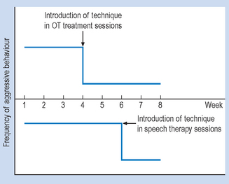
The hypothetical data presented in Figure 7.5 indicates that the frequency of the target behaviour (aggression) declined in Situation 1 when the intervention was introduced, while it remained stable in Situation 2. The subsequent introduction of the intervention in Situation 2 resulted in a decrease of the behaviour.
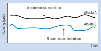
Multiple baseline designs can also be introduced by generating baselines for two or more behaviours, or for two or more individuals. Just as in the example involving the different situations, the interventions would be introduced first for one of the behaviours or individuals and, subsequently, for the others. Figure 7.6 illustrates a general example for multiple baseline designs.
Clearly, by introducing the intervention at different times, we are controlling for the effects of extraneous variables that might have influenced our dependent variable. Both ABAB and multiple baseline designs are appropriate for demonstrating the benefits of therapeutic procedures in individual patients.
The interpretation of the results for n = 1 designs
The principles for conducting and interpreting health research are also relevant for evaluating the effectiveness of everyday health practices. The need for control and accurate measurement arises when we intend to demonstrate that particular interventions or preventive interventions are causally related to beneficial outcomes.
As we have seen previously we can exercise control by systematically introducing and withdrawing interventions and measuring concomitant changes in the signs and symptoms of a disorder.
Hypothetical example
Let us examine a hypothetical example for illustrating four different methodological principles relevant to the interpretation of n = 1 studies. Imagine that you are caring for a young man called John who had suffered a severe fracture of the femur following a motorbike accident. He is gradually recovering with intensive rehabilitation but he is still in severe pain when narcotic analgesics are not provided.
Previous research has shown that transcutaneous electrical nerve stimulation (TENS) was a safe and effective modality for managing acute pain. However the intervention is not equally effective for all patients so that there are no absolute guarantees that TENS will control pain in this particular patient. Also, even biologically inert pain control techniques can reduce pain through placebo effects. In this case you decide to investigate two clinically relevant research questions:
Having obtained your patient’s informed consent you decide to conduct an ABAB, n = 1 design for obtaining evidence to answer the above research questions. The variables here can be defined as follows:
The therapeutic effectiveness of the TENS for pain control will be represented by the changes in the pain intensity or the differences between the A and B phases of the intervention. Table 7.1 provides the procedure for conducting the data collection.
Table 7.1 Data collection procedure for hypothetical example
| Time period | Independent variable level | Dependent variable |
|---|---|---|
| Week 1 | A phase (placebo) | Daily assessment of pain intensity (at 0800 hours) |
| Week 2 | B phase (treatment) | |
| Week 3 | A phase (placebo) | |
| Week 4 | B phase (treatment) |
The ‘A’ phase gives us the baseline against which we can compare the effectiveness of the active TENS intervention for reducing pain intensity. The outcome indicates a large and consistent difference between the A and B levels of the independent variable, and the large difference between A and B indicates a clinically useful reduction in the pain intensity experienced by John, your patient. You are now justified in continuing the intervention until he is sufficiently recovered to be painfree.
We hope you will agree that this was an inspiring little story, the problem with it being that things just do not normally happen this way in the real world. The data we hypothesized above clearly illustrate an ideal, easily interpreted outcome appropriate for educational purposes. However, there may be some factors in the real world that impact upon these idealized findings. These include:
The validity of n = 1 designs
We examined three (AB, ABAB, multiple baseline) designs in the previous subsections. However, more complicated, ‘mixed’ designs are available for n = 1 investigations. The mixed designs include elements of both reversal and multiple baseline strategies. We will not discuss these in detail in this text; interested readers are referred to Barlow & Hersen (1984).
A basic requirement for the valid interpretation of all n = 1 designs is the production of a stable baseline. Unless this requirement is met, the interpretation of the results is extremely difficult. In some clinical situations, the production of a stable baseline might be unethical as it could involve withholding treatment. The intervention phase must also be long enough for the effectiveness of the treatment to emerge. Some interventions, such as those involving physical rehabilitation or psychotherapy, might need to be administered for months before their effectiveness, or lack of it, becomes apparent. Clearly, we cannot assume that the baseline and intervention phases are of equal duration.
It is essential that the observations should be valid and reliable. Some observations are straightforward, such as those based on taking temperatures. However, given a more complex variable such as ‘aggression’ we need to establish with clarity that different observers agree on the type of behaviours we are going to observe; behaviours that might seem ‘aggressive’ to one observer might not be classified as such by another.
We have already discussed how n = 1 designs attempt to control for the influence of extraneous variables. Although the n = 1 designs can be conceptually adequate to demonstrate causality, the patients, being in their natural setting, can be influenced by all sorts of uncontrolled events. After all, it is not possible to insulate individuals from their environment. Therefore, sources of invalidity must be evaluated with respect to each n = 1 investigation. It must also be remembered that no matter how sophisticated the n = 1 design, the observed outcomes for any given case may not generalize to other cases.
Summary
In this chapter, we examined three (AB, ABAB and multiple baseline) of the designs available for studying single individuals in their natural settings. It was argued that ABAB and multiple baseline studies provide a valid means for evaluating the causal effects of variables on therapeutic outcomes. These n = 1 designs are particularly useful for establishing the usefulness of interventions for individual patients. Although some limitations and ethical constraints might emerge in conducting n = 1 studies, they provide a useful tool for practising health professionals interested in evaluating the effectiveness of their interventions.
Although the statistical analysis of n = 1 studies is beyond the scope of this introductory text, it should be noted that graphing our observations, as discussed in this chapter, provides evidence for possible causal relationships. A precondition for interpreting the results of n = 1 studies is having an adequate number of stable observations across the various conditions.
The n = 1 designs are quite similar to quasi-experimental designs, in that the investigator has control over the type and timing of the interventions.
Self-assessment
Explain the meaning of the following terms: