Chapter Fourteen Measures of central tendency and variability
Introduction
In the previous chapter we examined how raw data can be organized and represented by the use of statistics in order that they may be easily communicated and understood. The two statistics that are necessary for representing a frequency distribution are measures of central tendency and variability.
Measures of central tendency are statistics or numbers expressing the most typical or representative scores in a distribution. Measures of variability are statistics representing the extent to which scores are dispersed (or spread out) numerically. The overall aim of this chapter is to examine the use of several types of measures of central tendency and variability commonly used in the health sciences. As quantitative evidence arising from investigations is presented in terms of these statistics, it is essential to understand these concepts.
Measures of central tendency
The mode
When the data are nominal (i.e. categories), the appropriate measure of central tendency is the mode. The mode is the most frequently occurring score in a distribution. Therefore, for the data that was shown in Table 13.1 the mode is the ‘females’ category. The mode can be obtained by inspection of grouped data (with the largest group being the mode). As we shall see later, the mode can also be calculated for continuous data.
The median
With ordinal, interval or ratio scaled data, central tendency can also be represented by the median. The median is the score that divides the distribution into half: half of the scores fall under the median, and half above the median. That is, if scores are arranged in an ordered array, the median would be the middle score. With a large number of cases, it may not be feasible to locate the middle score simply by inspection. To calculate which is the middle score, we can use the formula (n + 1)/2, where n is the total number of cases in a sample. This formula gives us the number of the middle score. We can then count that number from either end of an ordered array.
In general, if n is odd, the median is the middle score; if n is even, then the median falls between the two centre scores. The formula (n + 1)/2 is again used to tell us which score in an ordered array will be the median. For example:
For a grouped frequency distribution, the calculation of the median is a little more complicated. If we assume that the variable is continuous (for example, time, height, weight or level of pain), we can use a formula for calculating the median. This formula (explained in detail below) can be applied to ordinal data, provided that the variable being measured has an underlying continuity. For example, in a study of the measurement of pain reports we obtain the following data, where n = 17:
The above data can be represented by a bar graph (Fig. 14.1).
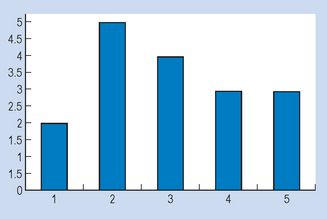
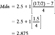
Here we can obtain the mode simply by inspection. The mode = 2 (the most frequent score). For the median, we need the ninth score, as this will divide the distribution into two equal halves (see Table 14.1). By inspection, we can see that the median will fall into category 3. Assuming underlying continuity of the variable and applying the previously discussed formula, we have:
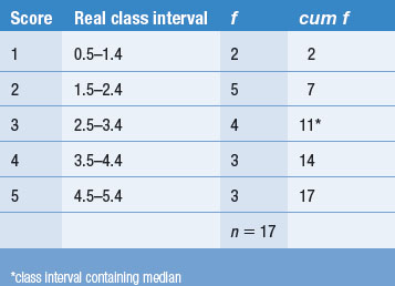
where XL = real lower limit of the class interval containing the median, i = width of the class interval, n = number of cases, cum fL = cumulative frequency at the real lower limit of the interval and fi = frequency of cases in the interval containing the median.
Substituting into the above equation:
The mean
The mean,  or μ, is defined as the sum of all the scores divided by the number of scores. The mean is, in fact, the arithmetic average for a distribution. The mean is calculated by the following equations:
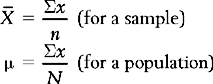
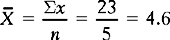
where Σx = the sum of the scores, = the mean of a sample, μ = the mean of a population, x = the values of the variable, that is the different elements in a sample or population, and n or N = the number of scores in a sample or population.
The formula simply summarizes the following ‘advice’:
To calculate the average or mean of a set of scores (), add together all the scores (Σx) and divide by the number of cases (n).
Therefore, given the following sample scores:
When n or N is very large, the average is calculated with the formula above but usually with the assistance of computers.
Comparison of the mode, median and mean
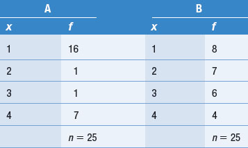
The mode can be used as a measure of central tendency for any level of scaling. However, since it only takes into account the most frequent scores, it is not generally a satisfactory way of presenting central tendency. For example, consider two sets of scores, A and B, shown in Table 14.2. It can be seen, either by inspection or by sketching a graph, that the two distributions A and B are quite different, yet the modes are the same, i.e. 1.
The median divides distributions into two equal halves, and is appropriate for ordinal, interval or ratio data. For interval or ratio data, however, the mean is the most appropriate measure of central tendency. The reason for this is that in calculating this statistic, we take into account all the values in the study sample. In this way, it gives the best representation of the average score. Clearly, it is inappropriate to use the mean with nominal data, as the concept of ‘average’ does not apply to discrete categories. For example, what would be the average of 10 males and 20 females?
There is some justification for using the median as a measure of central tendency when the variable being measured is continuous. However this is controversial, and the mean should be preferred. Alternatively, when a distribution is highly skewed, the median might be more appropriate than the mean for representing the ‘typical’ score. Consider the distribution:
Clearly, the median and the mode are less sensitive to extreme scores, while the mean is pulled towards extreme scores. This might be a disadvantage. For example, there are seven people working in a small factory, with the following incomes per week:
The distribution of wages is highly skewed by the high income of the owner of the factory ($1900). The mean, $500, is higher than six of the seven scores; it is in no way typical of the distribution. In cases like this the median is more representative of the distribution.
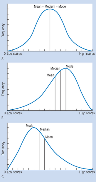
Figure 14.2 illustrates the relationships between the skew of frequency distributions and the three measures of central tendency discussed in this chapter. We should remember that the mode will always be at the highest point, the median will divide the area under the curve into halves, and the mean is the average of all the scores in the distribution. Also, the greater the skew in distribution, the more the measures of central tendency are likely to differ.
Measures of variability
We have seen that a single statistic can be used to describe the central tendency of a frequency distribution. This information is insufficient to characterize a distribution; we also need a measure of how much the scores are dispersed or spread out. The variability of discrete data is of little relevance, as the degree of variability will be limited by the number of categories defined by the investigator at the beginning of measurement.
Consider the following two hypothetical distributions representing the IQs of two groups of intellectually disabled children:
It is evident that although A= B = 60, the variability of the scores of Group A is greater than that of Group B. Insofar as IQ is related to the activities appropriate for these children, Group A will provide a greater challenge to the therapist working with the children.
The three statistics commonly used to indicate the numerical value of variability are the range, the variance and the standard deviation.
The range
The range is the difference between the highest and lowest scores in a distribution. As we mentioned, given the IQ data above, the ranges are:
Although the range is easy to calculate, it is dependent only on the two extreme scores. In this way, we are not representing the typical variability of the scores. That is, the range might be distorted by a small number of atypical scores or ‘outliers’. Consider, for instance, the differences in the range for the data given. The earlier example of the distribution of wages shows that just one outlying score in a distribution has an enormous impact on the range ($1900 − $100 = $1800). Obviously, some measure of average variability would be a preferable index of variability.
The average deviation
A convenient measure of variability might be average deviation about the mean. Consider Group B shown previously. Here = 60. To calculate the average variability about the mean, we subtract the mean from each score, sum the individual deviations, and divide by n, the number of measurements (see Table 14.3).
Table 14.3 Average variability about mean for Group B
| x | x − |
|---|---|
| 57 | −3 |
| 58 | −2 |
| 59 | −1 |
| 60 | 0 |
| 61 | +1 |
| 62 | +2 |
| 63 | +3 |
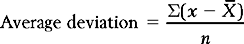
Therefore: Σ (x − ) = (− 3) + (− 2) + (− 1) + (0) + (1) + (2) + (3) = 0
This is a general result; the sum of the average deviations about the mean is always zero. You can demonstrate this for the average deviation of Group A. The problem can be solved by squaring the deviations, as the square of negative numbers is always positive. This statistic is called the sums of squares (SS) and is always a positive number. This leads to a new statistic called the variance.
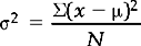
The variance
The variance (σ2 or s2) is defined as the sum of the squared deviations about the mean divided by the number of cases.
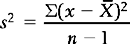
Divide by n − 1 when calculating the variance for a sample, when we use s2 as an estimate of population variance. Dividing by n results in an estimate which is too small, given that a degree of freedom has been lost calculating .
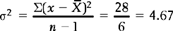
For the IQ example shown above, the variance is calculated as shown in Table 14.4.
Table 14.4 Calculation of variance
| x | x − |
(x − )2 |
|---|---|---|
| 57 | −3 | 9 |
| 58 | −2 | 4 |
| 59 | −1 | 1 |
| 60 | 0 | 0 |
| 61 | +1 | 1 |
| 62 | +2 | 4 |
| 63 | +3 | 9 |
|
= 60 |
Σ(x − )2 = 28 |
Substituting into the formula:
The problem with this measure of variability is that the deviations were squared. In this sense, we are overstating the spread of the scores. In taking the square root of the variance, we arrive at the most commonly used measure of variability for continuous data; the standard deviation.
The standard deviation
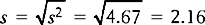
The standard deviation (σ or s) is defined as the square root of the variance:

Therefore, the standard deviation for Group B is:
The size of the standard deviation reflects the spread or dispersion of the frequency distribution representative of the data. Clearly, the larger σ or s, the relatively more spread out the scores are about the mean in a distribution. Calculation of the variance or the standard deviation is extremely tedious for large n using the method shown above. Statistics texts provide a variety of calculation formulae to derive these statistics. However, the common use of computers in research and administration makes it superfluous to discuss these calculation formulae in detail.
The semi-interquartile range
We have seen previously that if we are summarizing ordinal data, or interval or ratio data which is highly skewed, then the median is the appropriate measure of central tendency. The statistic called interquartile and semi-interquartile range is used as the measure of dispersion when the median is the appropriate measure of central tendency for a distribution. The interquartile range is the distance between the scores representing the 25th (Q1) and 75th (Q3) percentile ranks in a distribution.
It is appropriate to define what we mean by percentiles (sometimes called centiles). The percentile or centile rank of a given score specifies the percentage of scores in a distribution falling up to and including the score. As an illustration, consider Figure 14.3, in which:
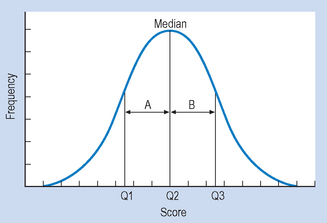
The distances A and B represent the distances between the median and Q1 and Q3. When a distribution is symmetrical or normal, the distances A and B will be equal. However, when a distribution is skewed, the two distances will be quite different. The semi-interquartile range (sometimes called the quartile deviation) is half of the distance between the scores representing the 25th (Q1) and 75th (Q3) percentile ranks in a distribution. Let us look at an example. If we have a sample where n = 16 and the values of the variable are:
clearly, a frequency distribution of these data is not even close to normal as the distribution is not symmetrical and the mode is at the maximum value. Therefore, the median is selected as the appropriate measure for central tendency, and we should use the interquartile range as the measure of dispersion.
Looking at the data, we find that:
where * denotes the 25th centile (first quartile, Q1), † denotes the 50th centile: median (second quartile, Q2) and ‡ denotes the 75th centile (third quartile, Q3).
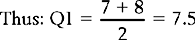
The score that cuts off the first 25% of scores (25th centile) is the first quartile (Q1). Since we have n = 16, Q1 will cut off the first four scores (25% of 16 is 4).
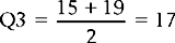
The third quartile (Q3) is the score which cuts off 75% of the scores. As n = 16, Q3 will cut off 12 scores (75% of 16 is 12).
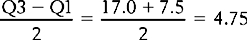
Therefore, the semi-interquartile range is:
The larger the semi-interquartile range, the more the scores are spread out about the median.
Summary
In this section, we discussed two essential statistics for representing frequency distributions: measures of central tendency and variability. The measures of central tendency outlined were the mode and median for discrete data, and the mean for continuous data. Measures of variability were shown to be the range, average deviation, variance, and standard deviation. These statistics are appropriate for crunching the data together to the point that the distribution of raw data can be meaningfully represented by only two statistics. That is, the raw data representing the outcome of investigations or clinical measurements are expressed in this manner. We have seen that the mean and the standard deviation are most appropriate for interval or ratio data. The median and semi-interquartile range are used when the data were measured on an ordinal scale, or when interval or ratio data are found to have a highly skewed distribution. The mode represents the most frequent scores. The contents of the chapter focused on the use and meaning of these concepts, rather than stressing calculations involved. These calculations are now made by computers. In Chapter 15, we discuss the application of the mean and standard deviation for relating specific scores to an overall distribution.
Self-assessment
Explain the meaning of the following terms:
True or false
Multiple choice
| No. of visits (x) | No. of patients (f) |
|---|---|
| 7 | 3 |
| 6 | 6 |
| 5 | 6 |
| 4 | 10 |
| 3 | 21 |
| 2 | 0 |
| 1 | 4 |