The Nerve
 Neuron
Functional anatomy
Neuron
Neuron, or the nerve cell, is the structural and functional unit of the nervous system. The nervous system of humans is made up of innumerable neurons. The total number of estimated neurons in the human brain is more than 1012. The neurons are linked together in a highly intricate manner. It is through these connections that the body is made aware of changes in the environment or of those inside the body itself; and appropriate responses to such changes are produced.
Structure
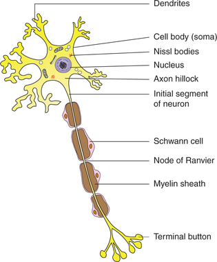
Neurons vary considerably in size, shape and other features. However, most of them have some major features in common. The basic structure of a neuron is best studied in a spinal motor neuron. A neuron primarily consists of the cell body and processes called neurites, which are of two kinds, the dendrites and the axon (Fig. 2.1-1).
Cell body
The cell body of a neuron is also called the soma or perikaryon and may be round, stellate, pyramidal or fusiform in shape. Like any other cell it consists of a mass of cytoplasm with all its principal constituents surrounded by a cell membrane. The cell body contains a large nucleus with one or two nucleoli but there is no centrosome. The absence of centrosome indicates that the neuron has lost its ability for division. Thus, neurons once destroyed are replaced by neuroglia only. In addition to the general features of a typical cell (page 8), the cytoplasm of a neuron has following distinctive characteristics (Fig. 2.1-1):
Nissl granules/bodies. These are basophilic granules that seem to be composed of rough surfaced endoplasmic reticulum. The Nissl bodies are present in the dendrites as well but are usually absent from the axon hillock and the axon.
Neurofibrillae. These consist of microfilaments and microtubules. In certain degenerative diseases like Alzheimer's disease, the neurofilament protein gets altered, resulting in the formation of neurofibrillary tangles.
Pigment granules are seen in some neurons. For example, neuromelanin is present in the neurons of substantia nigra. Aging neurons contain a pigment lipofuscin.
Dendrites
The dendrites are multiple, small branched processes. Dendrites contain Nissl bodies and neurofibrillae.
Dendrites are the receptive processes of the neuron receiving signals from other neurons via their synapses with axon terminals.
Axon
The axon is the single long process of the nerve cell. It varies in length from a few microns to a metre. It arises from the conical extension of the cell body called axon hillock, which is devoid of the Nissl bodies. The part of the axon between the axon hillock and the beginning of myelin sheath is called the initial segment. In the axon, the cell membrane continues as axolemma and the cytoplasm as axoplasm. The axon terminates by dividing into a number of branches, each ending in a number of synaptic knobs that are also known as terminal buttons or axon telodendria. Synaptic knobs contain microvesicles in which chemical neurotransmitters are stored. Myelin sheath is present around the axon in the so-called myelinated nerve fibres (Fig. 2.1-2).
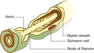
Fig. 2.1-2 Structure of a myelinated neuron. Note: Schwann cell encircles the axon to form myelin sheath.
Myelin sheath which consists of protein–lipid complex is produced by glial cells called Schwann cells which encircle the axons forming around it a thin sleeve. Each Schwann cell provides the myelin sheath for a short segment of the axon. At the junction of any two such segments there is a short gap, i.e. periodic 1 μm constrictions at about 1 mm distance. These gaps are the nodes of Ranvier. There are some axons which are devoid of myelin sheath.
Myelination of axons increases the speed of conduction, but greatly increases their diameter.
Axons perform the specialized function of conducting impulses away from the cell body. They transmit propagated impulses (all-or-none transmission).
Types of neurons
Neurons have been classified below on the basis of functions and myelination.
Depending upon the functions
Depending upon the functions the neurons are of two types: motor and sensory.
1. Motor neurons, also known as efferent nerve cells, carry the motor impulses from the CNS to the peripheral effector organs like muscles, glands and blood vessels. These neurons have very long axon and short dendrites.
2. Sensory neurons, also known as afferent nerve cells, carry the sensory impulses from the periphery to the CNS. These neurons have short axon and long dendrites.
Neuroglia
Neuroglia or the glial cells are the supporting cells present within the brain and spinal cord. They are numerous, about 10 times more than the neurons. Glial cells may be divided into two major categories (Fig. 2.1-3):
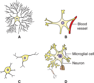
Fig. 2.1-3 Different types of glial cells: A, fibrous astrocyte; B, protoplasmic astrocyte; C, oligodendrocyte and D, microglial cells.
2 Microglia
Microglia or the small glial cells are mesodermal in origin. These are the smallest neuroglial cells having flattened cell body and short processes. They are more numerous in grey matter than in white matter. These act as phagocytes and become active after damage to nervous tissue by trauma or disease.
Peripheral nerve
A compact bundle of axons located outside the CNS is called a nerve. In a nerve the axons are arranged in different bundles called fasciculi (Fig. 2.1-4).
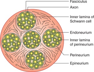
• Each axon or the nerve fibre is covered by endoneurium which is bounded internally by basal lamina around the Schwann cells and externally by the relatively impermeable inner basal lamina of the perineurium.
• Each fasciculus is covered by perineurium. The cells of the perineurium are tightly adherent and act as a barrier to the passage of particulate traces, dye molecules or toxins into the endoneurium.
• The whole nerve is covered by epineurium, which is a tubular sheath formed by an areolar membrane. It limits the extent to which the nerve can be stretched by body movements or external pressure, thereby protecting the fragile axons inside the nerve.
Biological activities
Protein synthesis
The cell bodies (soma) of all the neurons contain cellular apparatus required for the protein synthesis, i.e. the ribosomes and the Golgi apparatus. Since the axons do not have these organelles, all the proteins including the neurotransmitters are synthesized in the cell body and then transported along the axon to the synaptic knobs by the process of axoplasmic flow, as discussed below.
Axoplasmic transport
Axoplasm, the cytoplasm of the neurons is in constant motion. The axoplasmic transport is vital to nerve cell functions, since movements of various materials occur through it. The axoplasmic transport is of two types.
1 Anterograde transport
Anterograde transport, i.e. transport of materials away from the cell body. Some materials travel 100–400 mm a day along the axoplasm. Microtubules play an important role in this form of transport.
2 Retrograde transport
Retrograde transport, i.e. axoplasmic flow towards the cell body, may also carry tetanus toxin and neurotropic viruses (e.g. polio, herpes simplex and rabies) along the axon into the neuronal cell bodies in the CNS. It has also been employed by the neuroanatomists for charting out neural pathways.
Metabolism and heat production in the nerve fibres
Like other cells of the body, the metabolic activities occur in the nerve fibres as well; but the metabolism in nerve fibres occurs at a very low level. About 70% of the total energy required is used to maintain polarization of the membrane by the action of Na+–K+ ATPase pump. The energy is supplied mainly by combustion of sugars and phospholipids.
During nerve activity, the ATP and creatine phosphate breakdown, i.e. undergo hydrolysis and supply energy for the propagation of the nerve impulse.
Electrical properties of nerve fibre
The main electrical properties of the nerve fibres are:
• Excitability, i.e. the capability of generating electrical impulses (action potential).
• Conductivity, i.e. the ability of propagating the electrical impulses generated along the entire length of nerve fibres.
Excitability
Excitability is that property of the nerve fibre by virtue of which it responds by generating a nerve signal (electrical impulses or the so-called action potentials) when it is stimulated by a suitable stimulus which may be mechanical, thermal, chemical or electrical. In experimental studies, electrical stimulus is more frequently employed since its strength and frequency can be accurately controlled.
Before discussing the excitability (production of action potential), it will be useful to know about the electrical potential in the nerve fibre at rest, i.e. before it is stimulated (resting membrane potential).
Resting membrane potential
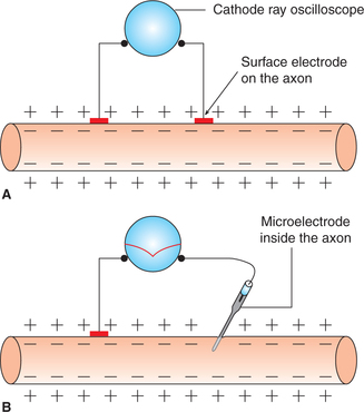
The study of electrical activity of a tissue has been made possible due to advances in the method of the recording electrical potentials, especially the development of microelectrodes and ‘cathode ray oscilloscope (CRO)’.
As shown in Fig. 2.1-5, when two electrodes are placed on the surface of a nerve fibre and connected to a CRO, no potential difference is observed. However, if one of the microelectrodes is inserted inside the nerve fibre (Fig. 2.1-5) a steady potential difference of −70 mV (inside negative) is observed on the CRO. This is resting membrane potential (RMP) and indicates the resting state of cell that is also called state of polarization. For details, see page 23.
Action potential
The action potential may be defined as the brief sequence of changes which occur in the resting membrane potential when stimulated by a threshold stimulus. When the stimulus is subminimal or subthreshold, it does not produce action potential, but does produce some changes in the RMP. There is slight depolarization for about 7 mV which cannot be propagated, since propagation occurs only if the depolarization reaches a firing level of 15 mV (−55 mV). Once the firing level is reached, there occurs action potential, i.e. there occurs abrupt depolarization with propagation (action potential).
Phases of action potential
The action potential basically occurs in two phases: depolarization and repolarization. When the nerve is stimulated, the polarized state (−70 mV) is altered, i.e. the RMP is abolished and the interior of the nerve becomes positive (+35 mV) as compared to the exterior. This is called depolarization phase. Within no time reverse occurs to the nearly original potential and this second phase of action potential is called repolarization phase.
Action potential curve is obtained when resting membrane potential is being recorded on a CRO and the nerve fibre is stimulated at a short distance away from the recording electrode (Fig. 2.1-6A) has following components (Fig. 2.1-6B):
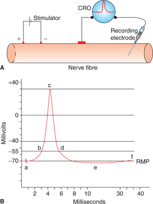
Fig. 2.1-6 Recording of action potential of a large mammalian myelinated nerve fibre: A, arrangement for recording action potential and B, various phases (components) of action potential. (a = Stimulus artefact, b = firing level, b–c = depolarization, c–d = repolarization, d–e = after depolarization, e–f = after hyperpolarization.)
1. Resting membrane potential is recorded as a straight baseline at −70 mV.
2. Stimulus artefact is recorded as a mild deflection of the baseline as soon as the stimulus is applied. The stimulus artefact occurs due to leakage of current from the stimulating electrode to the recording electrode.
3. Latent period is recorded as a short isoelectric period (0.5–1 ms) following the stimulus artefact. It represents the interval between the application of stimulus and the onset of action potential. It depends upon the distance between the site of stimulation, and the point of recording and the velocity of action potential along the particular axon.
4. Firing level. After the latent period, phase of depolarization starts. To begin with, depolarization proceeds relatively slow up to a level called the firing level (−55 mV), at which depolarization occurs very rapidly.
5. Overshoot. From the firing level, the curve reaches the zero potential rapidly and then overshoots the zero line up to +35 mV.
6. Spike potential. After reaching the peak (+35 mV), the phase of depolarization is completed and the phase of repolarization starts and the potential descends quickly near the firing level. The phase of rapid rise of potential in depolarization and a rapid fall in repolarization phase, combinedly constitute the so-called spike potential. Its duration is approximately 1 ms in an axon.
7. After depolarization is the slow repolarization phase which follows a rapid fall in spike potential and extends up to attainment of the RMP level. It is called phase of negative after potential and lasts for about 4 ms.
8. After hyperpolarization. After reaching the resting level (−70 mV) the potential further falls and becomes more negative (−72 mV). This phase is called after hyperpolarization or phase of positive after potential. It lasts for a prolonged period (35–40 ms). Finally, the RMP is restored.
Ionic basis of action potential
Role of voltage-gated Na+ and K+ channels
1. Polarization phase. Resting membrane potential (−70 mV) is due to distribution of more cations outside the cell membrane and more anions inside the cell membrane. At this point though Na+ are more in ECF, they cannot enter the cell due to the impermeability of the membrane.
2. Depolarization phase. When threshold stimulus is applied to the cell membrane, at the point of stimulation (Fig. 2.1-7), the permeability of the membrane for Na+ ions increases. At first the rise of permeability for Na+ is slow till it reaches the firing level. When the membrane depolarizes, the Na+ channels start opening up. The opening of the Na+ channels depolarizes the membrane further, leading to the opening of greater number of Na+ channels. As the concentration gradient and electrical gradient of this ion are directed inwards, there occurs a rapid influx of Na+ ions into the cell. This rapid entry of Na+ is sufficient to overwhelm the repolarizing forces.
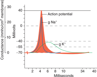
3. Repolarization phase. Repolarization occurs due to decrease in further Na+ influx and K+ efflux through the voltage-gated K+ channels which open later than Na+ channels but remain activated for prolonged period.
4. After depolarization. This is due to the fact that the rate of K+ efflux slows down as the electrical gradient responsible for initial rapid diffusion declines. This last phase of slow repolarization due to slow efflux of K+ is called after depolarization.
5. After hyperpolarization. The slow efflux of K+ con tinues even after the resting membrane potential is reached, resulting in a prolonged phase of hyperpolarization, during which the membrane potential falls up to −72 mV. However, little after, the voltage-gated K+ channels also shut down. The final ionic distribution is brought to the resting state by the action of Na+–K+ pump and the leak channels (K+, Cl−).
Characteristics of nerve excitability vis-a-vis characteristics of the stimulus
1 Strength–duration curve
The relationship between the strength and duration of a stimulus has been studied by varying the duration of a stimulus and finding out the threshold strength for each duration. The record of results plotted on a semilog graph paper gives the strength–duration curve (Fig. 2.1-8). Following inferences can be drawn from the strength–duration curve:
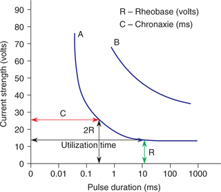
• Rheobase (R) refers to the minimum intensity of stimulus which if applied for adequate time (utilization time) produces a response.
• Chronaxie (C) refers to the minimum duration for which the stimulus of double the rheobase intensity must be applied to produce a response. Within limits, chronaxie of a given excitable tissue is constant. In other words, the chronaxie is an index of the excitability of a tissue and can be used to compare the excitability of various tissues. For example, a nerve fibre has far shorter chronaxie value than a muscle fibre indicating greater excitability of the former.
• When a stimulus of weaker intensity than the rheobase is applied, it will not produce a response, no matter how long the stimulus is applied.
• Stimulus of extremely short duration will not produce any response, no matter how intense that may be.
2 All-or-none response
A single nerve fibre always obeys ‘all-or-none law’, that is (Fig. 2.1-9):
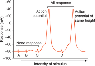
Fig. 2.1-9 All-or-none response in a single nerve fibre: A and B, represent subthreshold; C, threshold and D, suprathreshold stimuli.
• When a stimulus of subthreshold intensity is applied to the axon then no action potential is produced (none response).
• A response in the form of spike of action potential is observed when the stimulus is of threshold intensity.
• There occurs no increase in the magnitude of action potential when the strength of stimulus is more than the threshold level (all response).
This all-or-none relationship observed between strength of stimulus and response achieved is known as all-ornone law.
3 Membrane excitability during action potential
When a stimulus is applied to the nerve fibre membrane during the stage of action potential (produced by a previous threshold stimulus) then the response elicited depends upon the stage of action potential. Depend ing upon the response elicited to the stim ulus the period of action potential can be divided into: refractory period, supernormal period and subnormal period (Fig. 2.1-10).
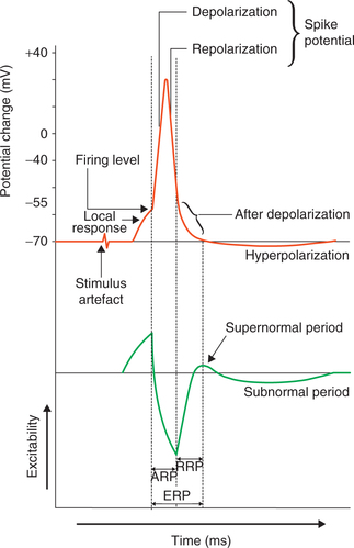
Fig. 2.1-10 Membrane excitability during different phases of action potential: ARP (absolute refractory period), RRP (relative refractory period) and ERP (effective refractory period).
(i) Refractory period
Refractory period refers to the period following action potential (produced by a threshold stimulus) during which a nerve fibre either does not respond or responds subnormally to a stimulus of threshold intensity or greater than threshold intensity. It is of two types:
(a) Absolute refractory period (ARP). It is a short period following action potential during which second stimulus, no matter how strong it may be, cannot evoke any response (another action potential). In other words, during absolute refractory period the nerve fibre completely loses its excitability. The absolute refractory period corresponds to the period of action potential from the firing level until repolarization is almost one-third complete (spike potential). During this period neither a fresh impulse can be generated, nor can an impulse generated elsewhere pass through this area.
Ionic basis of absolute refractory period. The Na+ channels are closed and slow potassium channels are not yet opened. Sodium channels do not open unless potential comes back to resting level. Therefore, during this period (absolute refractory period) the nerve fibre is not stimulated at all.
(b) Relative refractory period (RRP). It is a short period during which the nerve fibre shows response, if the strength of stimulus is more than normal. It extends from the end of absolute refractory period to the start of after depolarization of the action potential.
Ionic basis of relative refractory period. During this stage the Na+ channels are coming out of inactivated stage and voltage-gated potassium channels are still opened. The stronger stimulus (suprathreshold) at this stage is able to open more Na+ channels and thus excite a response. The action potential elicited during this period, however, has a lower upstroke.
4 Accommodation
We have studied that when a stimulus of sufficient strength (threshold level) is applied quickly, then the action potential is produced. However, when the stimulus strength is increased slowly to the firing level (during constant application), no action potential is produced. This phenomenon of adaptation to the stimuli is called accommodation. This is due to slow opening of Na+ channels and delayed closing of K+ channels. Thus repolarizing forces overwhelm depolarizing forces.
5 Infatiguability
A nerve fibre cannot be fatigued, even if it is stimulated for a long time. This property of infatiguability is due to the fact that during action potential neither a fresh impulse (action potential) can be generated nor the action potential can be conducted through the nerve fibre.
Electrotonic potential and local response
When a nerve fibre is stimulated by a subminimal or subthreshold stimuli then the action potential is not produced but there do occur some changes in the resting membrane potential. These local non-propagated changes are called electrotonic potentials or acute subthreshold potentials.
Types of electrotonic potentials
Depending upon the nature (negative or positive) of subthreshold level current used to stimulate (Fig. 2.1-11), the electrotonic potentials are of two types:
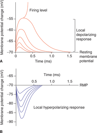
1. Catelectrotonic potential. Catelectrotonic potentials are localized depolarizing potential changes in the membrane potential produced when the stimulus of subthreshold strength is applied with cathode. This potential change rises sharply and then decays exponentially with time.
2. Anelectrotonic potential. Anelectrotonic potentials are the localized hyperpolarizing potential changes in the membrane potential when anodal subthreshold current is applied.
Graded potentials
As shown in Fig. 2.1-11, the electrotonic potentials produced by varying intensities of stimuli are proportionate to the magnitude of stimulation. Therefore, these are also known as graded potentials. The graded response is achieved both at cathode and anode up to 7 mV of depolarization or hyperpolarization.
Differences between graded potentials and action potential are summarized in Table 2.1-1.
Table 2.1-1
Differences between graded potential and action potential
| Graded potential | Action potential |
| 1. The amplitude of graded potential is proportionate to the intensity of the stimulus and can get summated. | The amplitude of action potential remains constant with increasing intensity of stimulus, therefore it cannot be summated. |
| 2. Graded potentials can be either depolarizing or hyperpolarizing. | Action potential is always depolarizing. |
| 3. Graded potential can be generated either spontaneously or in response to either physical or chemical stimuli. | Action potential is generated only in response to membrane depolarization. |
| 4. Graded potentials cannot conduct impulse. | Action potential can conduct impulses. |
| 5. Examples are: • Receptor potential at sensory nerve endings. • Motor end plate potential. |
Examples are: • Action potential of a nerve fibre, skeletal muscle and cardiac muscle. |
Inhibition of excitability
There are certain factors which inhibit the excitability of the nerve fibres. Some of the factors or the conditions which lead to inhibition or decrease in excitability are given below.
1. High extracellular calcium concentration. A high extracellular Ca2+ concentration decreases membrane permeability to Na+ ions thereby decreasing the membrane excitability.
2. Local anaesthetics. Local anaesthetic agents like procaine, tetracaine and lidocaine block the Na+ channels thus reduce the membrane excitability.
Conductivity
Conductivity refers to the propagation of nerve impulse (action potential) in the form of a wave of depolarization through the nerve fibre. Mechanism of conduction of action potential along an unmyelinated nerve fibre and a myelinated nerve fibre is described below.
Propagation of action potential in an unmyelinated axon
The steps of propagation of action potential along an unmyelinated axon are summarized:
• In the resting phase (polarized state), the axonal membrane is outside positive and inside negative (Fig. 2.1-12A).
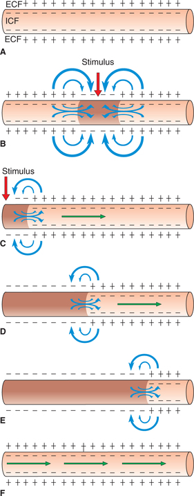
Fig. 2.1-12 Electrotonic conduction of impulse in an unmyelinated nerve fibre: A, resting phase (polarized state); B, conduction of impulse in both directions when stimulus applied at the middle of nerve fibre; C, when stimulus applied at one end of the nerve fibre; D and E, propagation of impulse in one direction along the nerve fibre and F, repolarization (occurs in same direction).
• When an unmyelinated axon is stimulated at one site by a threshold stimulus, there occurs action potential at that site, i.e. that site is depolarized. In other words, at that site outside becomes negative and inside positive (reversal of polarity) but the neighbouring areas until now remain in polarized state (Fig. 2.1-12C).
• As ECF and ICF are both conductive to electricity, a current will flow from positive polarized area to negative activated area through the ECF and in the reverse direction in the ICF (Fig. 2.1-12C). Thus, a local circuit current flows between the resting polarized site to the depolarized site of the membrane (current sink).
• This circular current flow depolarizes the neighbouring area of the membrane up to the firing level, and a new action potential is produced which in turn depolarizes the neighbouring area ahead. Thus, due to successive depolarization of the neighbouring area, the action potential is propagated along the entire length of the axon (Fig. 2.1-12D). This type of conduction is known as electrotonic conduction. Once initiated, the moving impulse cannot spread to reverse direction because the proximal site is in refractory state and thus the distal sites being in polarized state keep on getting depolarized. Thus, the direction of propagation of impulse is that of current flow inside the nerve fibre (Fig. 2.1-12E).
• The depolarization remains at any site for some length of time; therefore, portion which depolarizes first also repolarizes first. Thus, the repolarization is also propagated following the depolarization (Fig. 2.1-12F).
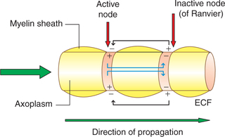
Propagation of action potential in a myelinated axon
The myelinated nerve fibres have a wrapping of myelin sheath with gaps at regular intervals which are devoid of myelin sheath (nodes of Ranvier). The myelin sheath acts as an insulator and does not allow the current flow. Therefore, in myelinated nerve fibres the local circuit of current flow only occurs from one node of Ranvier to the adjacent node (Fig. 2.1-13). That is, the impulse (action potential) jumps from one node of Ranvier to next. This is known as saltatory conduction. Since the impulse jumps from one node to other, the speed of conduction in the myelinated fibres is much rapid (50–100 times faster) than the unmyelinated fibre.
Orthodromic versus antidromic conduction
Normally, the action potential is propagated in one direction. That is, usually the nerve impulse from the receptors or synaptic junctions travels along the entire length of axon to their termination. This type of conduction is called orthodromic conduction. The conduction of nerve impulse in the opposite direction, as seen in the sensory nerve supplying the blood vessels, is called antidromic conduction.
Conduction velocity
Factors affecting conduction velocity
The velocity of conduction in the nerve fibres varies from as little as 0.25 m/s in very small unmyelinated fibres to as high as 100 m/s in very large myelinated fibres. In general, the factors affecting conduction velocity are as follows.
1. Temperature. A decrease in temperature delays conduction, i.e. slows down the conduction velocity.
2. Axon diameter affects the conduction velocity through the resistance offered by the axoplasm (Ri) to the flow of axoplasmic current. If the diameter of the axon is greater, the axoplasmic resistance (Ri) is lesser and hence the velocity of conduction is higher.
3. Myelination increases conduction velocity by its following effects:
Recording of membrane potential and action potentials
The recording of membrane excitation and action potential is made possible by the use of highly sophisticated equipment. The mammalian axons are about 20 μm or less in diameter; so being relatively small, it is very difficult to separate them out from other axons. Certain invertebrate species like crab (carcinus), cuttlefish (sepia) and squid (loligo) have giant cells. The largest axon found in the neck region of loligo is about 1 mm in diameter. The fundamental properties are quite similar to the human axons. Therefore, these animals can be used for recording various events.
Instruments used for recording
The essential instruments used in recording the activity of excitable tissue are:
Basic principles of the functioning of these instruments are discussed briefly.
1 Microelectrodes
The microelectrodes are usually very small pipette (micropipette) of tip size less than 1 μm diameter. The tip of micropipette electrode is impaled through the cell membrane of the nerve fibre. Another electrode called indifferent electrode is placed in the extracellular fluid (Fig. 2.1-14).
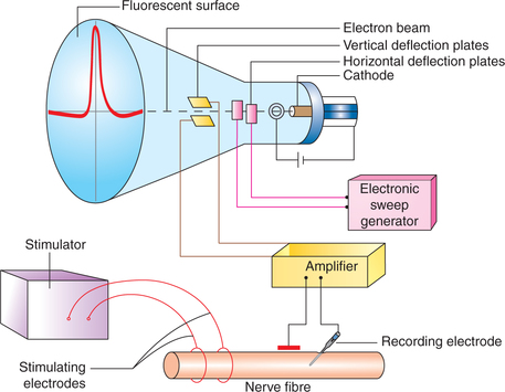
Fig. 2.1-14 Cathode ray oscilloscope and simplified diagram to record action potential from a nerve fibre.
The microelectrode can be connected to the cathode ray oscilloscope through a suitable amplifier for recording rapid changes in membrane potential during nerve impulse transmission.
2 Electronic amplifier
This device can magnify the potential changes of the tissue to more than thousand times so that these can be recorded on the oscilloscope screen.
3 Cathode ray oscilloscope
Cathode ray oscilloscope (CRO) is almost an inertialess instrument which can record and measure the electrical events of living tissues instantaneously. The CRO primarily consists of a glass tube with a cathode, fluorescent surface (screen) and two sets of electrically charged plates (Fig. 2.1-14).
Cathode is in the form of an electronic gun. When connected to a suitable anode and electric current, the electronic gun emits electrons.
Fluorescent surface (the face of glass tube coated with fluorescent material) acts as a screen. The electrons emitted from the cathode are directed into a beam which hits this screen.
Electrically charged plates are arranged in two sets: vertical and horizontal
• Horizontal deflection plates are placed on either side of the electron beam. These are connected to sweep generator (electronic sweep circuit). When a voltage is applied across these plates the beam of electrons (being negatively charged) is attracted towards the positively charged plate and repelled away by the negatively charged plate. If saw-tooth voltage (i.e. voltage is increased slowly, then suddenly reduced, and again slowly increased) is applied then the electron beam will steadily move towards the positively charged plate (with slowly increasing voltage), then back to its original position (with sudden reduction in the voltage) and then again move towards the positively charged plate. In this way the electron beam is made to sweep across the fluorescent screen horizontally, which will give a continuous marking of line of glowing light.
• Vertical deflection plates are placed above and below the electron beam. These are connected to recording electrodes placed on the nerve through an electronic amplifier. The potential change occurring in the nerve will charge these plates, which will cause vertical (upward and downward) deflection of the electron beam. The magnitude of deflection will be proportional to the potential difference between the two plates. Thus action potential is recorded as vertical deflection of the beam as it moves across the fluorescent screen of the CRO.
Recording of resting membrane potential
The arrangement of electrodes for recording membrane potential is shown in Fig. 2.1-15. The electrical potential is recorded at the surface of the membrane (exterior) and inside the membrane at each point in a nerve fibre. Starting from one end of the nerve fibre (left side of the figure) and passing to the other end (right side) and when both the electrodes (indifferent and microelectrodes) are on the surface (outside) of the nerve fibre membrane, then no potential difference was recorded (zero potential), which is potential of extracellular fluid. However, when microelectrode is made to penetrate into the interior of cell, a constant potential difference (–70 mV) is observed. This is known as resting membrane potential (Fig. 2.1-15).
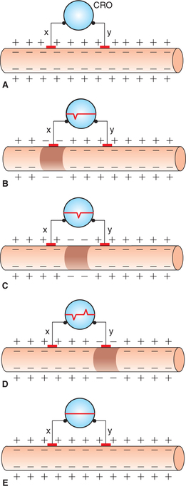
Fig. 2.1-15 Arrangement for recording biphasic action potential (recording electrodes x and y are on the surface of nerve fibre connected to cathode ray oscilloscope): A, resting state; B, on stimulation when wave of excitation reaches at electrode ‘x’; C, when impulse passes beyond electrode ‘x’; D, when impulse reaches at electrode ‘y’ and E, when impulse passes away from electrode ‘y’.
Recording of action potential
Monophasic recording of action potential
For monophasic recording of action potential, one microelectrode is placed inside the nerve fibre and the other electrode on the outside surface. These electrodes are then connected to the cathode ray oscilloscope (Fig. 2.1-14). When the nerve is stimulated a typical monophasic record of action potential obtained has the following components:
It has been described in detail on page 32.
Biphasic recording of action potential
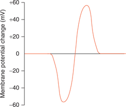
For biphasic recording of action potential, both the exploring electrodes (x and y) are placed on the outside surface of nerve fibre and are connected to a CRO (Fig. 2.1-15). When nerve is stimulated, the excitation of one electrode causes deflection opposite to that of another during the passage of impulse. Record of this alternate deflection of one negative below the baseline and one positive above the baseline (called biphasic action potential) is depicted (Fig. 2.1-16).
Compound action potential
Compound action potential is the monophasic recording of action potential from a mixed nerve, which contains different types of nerve fibres with varying diameter. Therefore, the compound action potential represents an algebraic summation of the all-or-none action potentials of many axons.
Response of a mixed nerve to stimulus
Response of a mixed nerve to a stimulus will depend upon the thresholds of the individual axon in the nerve and their distance from the stimulating electrode (Fig. 2.1-17):
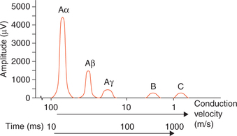
Fig. 2.1-17 Typical record of compound action potential (recorded from a mixed nerve) showing multiple peaks.
Features of a compound action potential.
• It has a unique shape (multiple peaks) because a mixed nerve is made up of different fibres with various speeds of conduction.
• The number and size of the peaks vary with the types of fibres in the particular nerve being studied.
• When less than maximal stimuli are used, the shape of compound action will depend upon the number and type of fibres stimulated.
Nerve fibre types
Various schemes for classification of the nerve fibres on the basis of their diameter and their conduction velocity have been proposed.
Classification of nerve fibres
1 Letter classification of Erlanger and Gasser
This is the best known classification based on the diameter and conduction velocity of the nerve fibres. The nerve fibres have been classified as follows:
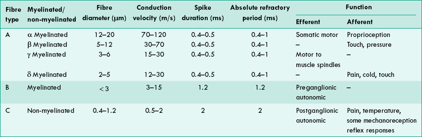
‘Type A’ nerve fibres. The fastest conducting fibres are called type A fibres. Their diameter varies from 12–20 μm and conduction velocity from 70–120 m/s. They are myelinated fibres.
Type A fibres have been further subdivided into α, β, γ and δ. Type A fibres subserve both motor and sensory functions.
‘Type B’ nerve fibres. These fibres are myelinated, have a diameter of less than 3 μm and their conduction velocity varies from 4–30 m/s. They form preganglionic autonomic efferent fibres, afferent fibres from skin and viscera, and free nerve endings in connective tissue of muscle.
‘Type C’ nerve fibres. These are unmyelinated, have a diameter of 0.4–1.2 μm and their conduction velocity varies from 0.5–4 m/s. These form the postganglionic autonomic fibres, some sensory fibres carrying pain sensations, some fibres from thermoreceptors and some from viscera. The salient features of type A, B and C nerve fibres are summarized in Table 2.1-2.
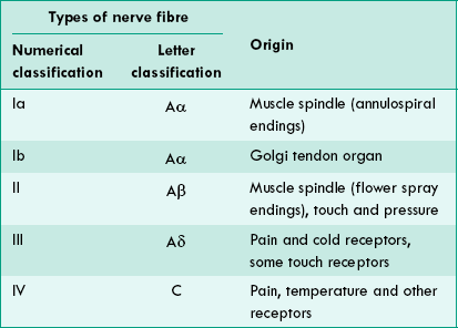
2 Numerical classification
Some physiologists have classified sensory nerve fibres by a numerical system into type Ia, Ib, II, III and IV. A comparison of the numerical classification and the letter classification is shown in Table 2.1-3.
3 Susceptibility of nerve fibres to hypoxia, pressure and local anaesthetics
Hypoxia. As shown in Table 2.1-4, the type B fibres are most susceptible to hypoxia.
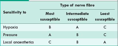
Pressure. Type A fibres are most susceptible to pressure and type C least.
Local anaesthetics. Type C fibres (conducting pain, touch and temperature sensations generated by cutaneous receptors) are most susceptible to local anaesthetics. This fact is useful for surgical interventions under local anaesthesia.
Degeneration and regeneration of neurons
When the axon of neuron is injured, a series of degenerative changes are seen at three levels:
Along with the degenerative changes, the reparative process (regeneration) also starts soon if the circumstances are favourable. The effects of injury to a nerve and the occurrence of regenerative changes thereafter will depend upon the degree and type of damage.
Stage of degeneration
The degenerative changes which occur in the part of axon distal to the site of injury are referred to as an anterograde degeneration or Wallerian degeneration (after the discoverer A Waller, 1862). The degenerative changes occurring in the neuron proximal to the injury are referred to as retrograde degeneration. These changes take place in the cell body and in the axon proximal to injury.
Changes in the part of axon distal to injury
The degenerative changes start within few hours of injury and continue for about 3 months and include the following (Fig. 2.1-18).
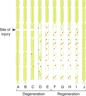
Fig. 2.1-18 Degenerative changes (Wallerian degeneration) in distal part of a nerve fibre after injury (A–E) and subsequent regenerative changes (F–J).
Axis cylinder
Axis cylinder becomes swollen and irregular in shape within a few hours of injury. After a few days it breaks up into small fragments, the neurofibrils within it break down into granular debris and are seen in the space occupied by axis cylinder.
Changes in the cell body of neuron
Changes in the cell body of injured neuron start within 48 h and continue up to 15–20 days. The changes are discussed below.
Nissl substances undergo disintegration and dissolution (chromatolysis).
Golgi apparatus, mitochondria and neurofibrils are fragmented and eventually disappear.
Cell body draws in more fluid, enlarges and becomes spherical.
Nucleus is displaced to the periphery (towards cell membrane). Sometimes the nucleus is extruded out of the cell, in which case the neuron atrophies and finally disappears completely.
Stage of regeneration
The stage of degeneration is followed by the stage of regeneration under favourable circumstances (listed below). It starts within 4 days of injury but becomes more active after 30 days, and may take several months to a year for complete recovery.
Factors affecting regeneration
• Regeneration occurs more rapidly when a nerve is crushed than when it is severed and the cut ends are separated.
• Chances of regeneration of a cut nerve are considerably increased if the two cut ends are near each other (gap does not exceeds 3 mm) and remain in the same line.
• Presence of neurilemma is a must for regeneration to occur. Therefore, axons in the CNS once degenerated never regenerate as these nerve fibres have no neurilemma.
• Presence of nucleus in the neuron cell body is also must for regeneration to occur. If it is extruded, the neuron is atrophied and the regeneration does not occur.
Regenerative changes
Anatomical regeneration
Stage of fibres formation. Axis cylinder from the proximal cut end of the axon elongates and gives out fibrils up to 100 in number in all directions. These branches grow into the connective tissue at the site of injury in an effort to reach the distal cut end of the nerve fibre (Fig. 2.1-18F and Fig. 2.1-18G).
Stage of entry of fibrils into endoneural tube. Strands of the Schwann cells from the distal cut end of axon guide the regenerating fibrils to enter their axon endoneural tube, once the fibril enters the endoneural tube it grows rapidly within it. The axonal fibrils that fail to enter one of the tubes degenerate.
Stage of active growth. The axonal fibril growing through the endoneural tube enlarges and establishes contact with an appropriate peripheral end organ. The new axon formed in this way is devoid of myelin sheath (Fig. 2.1-18H and Fig. 2.1-18I). The process of regeneration up to this stage takes about 3 months.
Stage of myelination. The myelin sheath is then formed by the cells of Schwann slowly. The myelination is completed in 1 year.