Chapter 8 Pharmacokinetics and Dosing Regimens
The choice of a drug for an individual patient is influenced by many factors, and using the correct dose is essential both for achieving the desired pharmacological effect and for limiting adverse effects. An understanding of pharmacokinetic principles allows selection of the right dose and the prediction of the effects of disease states, drug interactions and environmental factors on dosing regimens. The importance of the key pharmacokinetic concepts of clearance, volume of distribution and half-life are illustrated in this chapter by the use of examples relevant to the clinical situation.
Key abbreviations
AUC area under the plasma concentration versus time curve
RATIONAL use of drugs is based on the assumption that a particular concentration of a drug will have the desired therapeutic effect and that adverse effects will be negligible. For many drugs there is a sufficient relationship between plasma drug concentration and clinical response for dosing regimens to be designed to maintain the concentration within a therapeutic range. Although therapeutic ranges are derived from data on populations of individuals, not everyone responds in the same way. Some individuals might not experience a therapeutic effect when the plasma drug concentration is at the top of the range, and others might experience toxicity when the plasma drug concentration is within the therapeutic range. The therapeutic range is generally considered to reflect the range of drug concentrations having a high probability of producing the desired therapeutic effect and a low probability of producing adverse effects. For a limited number of drugs it is possible to individualise the dosing regimen to achieve the desired plasma concentration for an individual by considering their characteristics (e.g. age, health status, liver and kidney function) and the pharmacokinetics of the drug.
After administration, each drug will have its own characteristic pharmacokinetic profile that is influenced by factors such as the route of administration, changes in the disease state of the individual, the person’s genetic make-up and environmental factors. Despite these potential confounding factors, in general the aim is to achieve a constant (steady-state) plasma drug concentration that maintains the desired pharmacological response. This can be achieved through continuous administration (e.g. IV infusion) or through multiple dosing via other routes, most commonly the oral route. The size of the dose and the dosing frequency constitute a dosing regimen. As can be appreciated from Chapter 6, pharmacokinetics plays a major role not only in establishing the initial dosing regimen but also in adjusting the regimen to deal with a lack of response or to reduce symptoms of toxicity.
Plasma concentration–time profile of a drug
Measuring the plasma concentration–time profile of a drug demonstrates graphically the relationship between the plasma drug concentration and therapeutic response or toxicity over time. For example, the theoretical drug in Figure 8-1 has been administered as a single oral dose. It has an onset of action of approximately 2 hours, a peak plasma concentration at 5 hours, and a 6-hour duration of action (the length of time the plasma drug concentration remains within the therapeutic range). In this case the processes of absorption, distribution and elimination (i.e. metabolism and excretion) influence the plasma concentration–time profile of the drug.
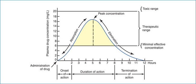
Figure 8-1 Plasma concentration–time profile for a theoretical drug administered as a single oral dose.
Administration of a drug by the IV route as a single bolus dose followed by an infusion, as a single bolus dose alone or as an infusion alone all give different plasma concentration–time profiles that are influenced by distribution and elimination but not absorption (Figure 8-2).
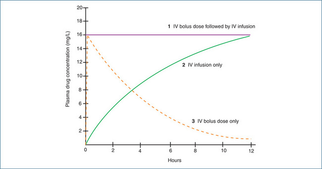
Figure 8-2 Plasma concentration–time profiles for a drug administered as (1) a single IV bolus dose followed by an IV infusion, (2) an IV infusion only, and (3) a single IV bolus dose.
How does this knowledge help you to design an appropriate dosing regimen? Buried within these plasma drug concentration–time profiles are the key pharmacokinetic parameters of clearance, volume of distribution and half-life. The clearance of a drug and its volume of distribution are determined by the characteristics of both the patient and the drug, whereas the plasma half-life of the drug is a composite parameter that is related directly to the volume of distribution of the drug and inversely to the clearance of the drug. Each of these parameters will be discussed in the following sections in the context of their clinical relevance.
Area under the plasma concentration versus time curve
The area under the plasma concentration versus time curve (AUC) is exactly what the phrase implies. It can be used to calculate both the clearance of a drug after IV administration and the bioavailability of a drug (see Chapter 6). The latter is calculated by comparing the respective AUC values after IV and oral administration of the same dose of the same drug.
The AUC is defined as the ‘total area under the curve that describes the concentration of the drug in the systemic circulation as a function of time post dose (normally zero until infinity)’. The value of AUC is obtained by dividing the area under the curve into equal-sized strips, then estimating the area of each strip as that of a trapezium, then adding up all the results. This is commonly called ‘the trapezoidal rule’ and is illustrated in Figure 8.3. Generally, the larger the AUC, the smaller the clearance, because of the relationship
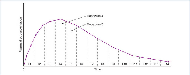
Figure 8-3 Plasma drug concentration versus time curve after an oral dose of a drug. The AUC is determined by calculating the area of each trapezium and summing the values. AUC = Area T1 + Area T2 + Area T3 + Area T4 … + Area Tn

The AUC may also be used to determine the absolute bioavailability of a drug (Chapter 6). Usually a group of subjects will be given the same IV and oral dose of the same drug on separate occasions. After each drug dose, blood samples are collected for many hours (e.g. at least 2–3 half-lives). The plasma concentration versus time curve is plotted for both the IV and the oral dose and the AUC is calculated for each curve. Fortunately most pharmacokinetic programs calculate the AUC automatically, and manual calculation by the trapezoidal rule is not necessary! As the bioavailability of an IV dose is 100% by definition, if the AUC of the oral dose is half of the AUC of the IV dose, then the bioavailability of the oral formulation is 50%.
Box 8-1 Key pharmacokinetic definition: clearance
Clearance (CL) is the volume of blood cleared irreversibly of drug per unit time. Clearance has units of flow (volume/time) and is expressed as either litres per hour (L/h) or millilitres per minute (mL/min).
Note: The factor for converting mL/min to L/h is 60/1000, i.e. 0.06. The factor for converting L/h to mL/min is 1000/60, i.e. 16.67.
Key pharmacokinetic concept—clearance
Clearance (CL) describes the ability of either an individual organ or the body to eliminate a drug. Clearances by each organ are additive and, hence, total clearance from the systemic circulation (CLS) reflects the total sum of all the clearance processes relevant to the particular drug (Figure 8-4). For example:
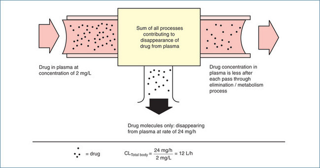
Figure 8-4 Concept of total body clearance of a drug from plasma. Only some drug molecules disappear from plasma on each pass of blood through kidneys, liver or other sites contributing to drug disappearance (elimination). In this example, it requires 12 L plasma to account for the amount of drug disappearance each hour (24 mg/h) at the concentration of 2 mg/L. Total body clearance is thus 12 L/h.
Source: Brody et al 1998. Reproduced with permission.

In general, for most drugs unless indicated otherwise, CL by other organs (e.g. the lungs) is usually neglected. For a particular drug and a specific individual, providing they remain physiologically stable, CL is constant. For example, if you measured the CL of paracetamol in yourself it should not change very much from day to day, provided the activity of your liver enzymes that metabolise paracetamol did not change. However, paracetamol CL in a population of individuals will broadly reflect the interindividual variability in the activity of drug-metabolising enzymes.
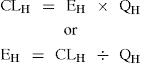
CL is also defined mathematically and the rate at which a drug is eliminated from the body varies directly with the plasma drug concentration (C).

If you clear drug X at a constant rate of 10 L/h and the plasma concentration of drug X is 20 mg/L, the elimination rate of drug X is 200 mg/h. If the concentration of drug X drops to 10 mg/L, the elimination rate becomes 100 mg/h.
Hepatic clearance
If a drug is described as having a hepatic clearance (CLH) of 30 L/h, what does this mean if hepatic blood flow is 90 L/h? It does not mean that the liver irreversibly removes (clears) drug from only 30 L of blood and not from the other 60 L of blood that passes through it. What it does mean is that one-third (30/90) of the drug molecules entering the liver in blood are cleared by the liver in one pass. Hepatic clearance of drug occurs mainly as a result of metabolism and in this case the capacity of the drug-metabolising enzymes is such that only one-third of the drug is removed from the blood. If the drug was not metabolised at all, hepatic clearance would be zero; conversely, if all the drug entering the liver was metabolised in a single pass then clearance would equal hepatic blood flow, 90 L/h.
In Chapter 6 the concept of hepatic extraction was introduced in relation to bioavailability; here we discuss it in terms of hepatic clearance.
For a drug to be cleared (metabolised) it has to be delivered to the liver and CLH also depends on liver blood flow (90 L/h), which is given the symbol QH. Hepatic
Box 8-2 Key pharmacokinetic definition: hepatic extraction ratio (EH)
Hepatic extraction ratio (EH) is defined as ‘the fraction of the drug entering the liver in blood that is irreversibly removed (or extracted) by metabolism on each pass through the liver. EH ranges from 0 when no drug is extracted to 1 when all the drug is extracted’. In Figure 6-4 in Chapter 6, EH was 0.75
clearance (CLH) is the product of the hepatic extraction ratio (EH) and liver blood flow (QH).
If we consider two drugs, and drug Z has a CLH of 80 L/h and drug Y has a CLH of 2 L/h and QH is 90 L/h, we can calculate the extraction ratios.
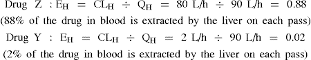
If we assume absorption was complete (that is fg = 1), the bioavailability of drug Z is 12% and of drug Y is 98%.
Drugs metabolised by the liver are classified according to the relationship between CLH and QH as having low, intermediate or high hepatic clearance.
Examples of drugs in these categories are shown in Table 8-1. Low hepatic clearance does not mean that the drug is then cleared by the kidneys; it indicates that the capacity of the hepatic enzymes involved in the metabolism of the drug is low.
Table 8-1 Examples of drugs with low, intermediate and high hepatic clearances
| Low hepatic clearance | Intermediate hepatic clearance | High hepatic clearance |
| Carbamazepine | Caffeine | Lignocaine |
| Diazepam | Fluoxetine | Morphine |
| Ibuprofen | Midazolam | Pethidine |
| Phenytoin | Omeprazole | Propranolol |
| Warfarin | Paracetamol | Zidovudine |
Effect of enzyme induction and inhibition on hepatic clearance
In Chapter 6 the effects of enzyme induction and inhibition on drug metabolism were discussed. In considering CLH how relevant are induction and inhibition to low and high hepatic clearance drugs and their respective oral bioavailabilities? The following examples illustrate the effects of enzyme induction and inhibition; in each example liver blood flow is assumed to be 90 L/h and absorption (fg) is 1.
Induction of metabolism
Example 1 Drug A: A high hepatic clearance drug with EH = 0.8

If another drug is administered that induces metabolism, increasing EH to 0.9

Although hepatic clearance of drug A was changed minimally by hepatic enzyme induction, the effect on bioavailability was substantial, that is, a reduction from 20% to 10%, and hence the systemic blood concentration will be reduced accordingly.
Example 2 Drug B: A low hepatic clearance drug with EH = 0.01

If another drug is administered that induces metabolism increasing EH to 0.02

For drug B a doubling of hepatic clearance has resulted in a clinically insignificant effect on bioavailability.
Inhibition of metabolism
If we use drug A and drug B again but instead administer another drug that inhibits hepatic metabolism and decreases EH by 20% what is the outcome on bioavailability for each drug?
Example 3 Drug A: A high hepatic clearance drug with EH = 0.8 prior to administration of the inhibiting drug

For drug A, a high hepatic clearance drug, inhibition of metabolism has had a significant effect on bioavailability (increased from 20% to 36%), and hence the systemic blood concentration will be increased accordingly.
Example 4 Drug B: A low hepatic clearance drug with EH = 0.01 prior to administration of the inhibiting drug

For drug B a 20% reduction in hepatic clearance has resulted in a clinically insignificant effect on bioavailability.
From these examples it can be seen that although the systemic clearance of high clearance drugs is relatively unaffected by changes in drug-metabolising enzyme activity, changes in enzyme activity will affect bioavailability of high clearance drugs (Examples 1 and 3). In contrast, with low hepatic clearance drugs changes in EH significantly alter hepatic clearance but have a negligible effect on bioavailability (Examples 2 and 4). Clinically the impact of enzyme induction or enzyme inhibition will depend on the drug and the metabolising enzyme(s). This will be discussed further in Chapter 10 when we consider drug–drug interactions.
Renal clearance
The kidneys are the major organs for the clearance of polar water-soluble drugs. Renal drug clearance is the net effect of glomerular filtration, secretion and passive reabsorption. Examples of drugs principally cleared by the kidneys include the penicillin and cephalosporin antibiotics. For most drugs, changes in renal function do not always necessitate an adjustment in drug dosage. However, when renal function is reduced to less than half and the drug is more than 50% cleared by the kidneys, dosage adjustment is necessary. Digoxin and gentamicin are examples of drugs cleared by the kidneys and for which the dosing regimen needs to be changed in individuals with renal impairment.
The importance of clearance
Continued drug administration eventually leads to a situation in which the rate of drug in equals the rate of drug out and the plasma drug concentration remains constant.
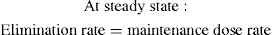
Box 8-3 Key pharmacokinetic definition: steady state
At steady state, the rate of drug administration equals the rate of drug elimination.
Clearance (CL) determines the maintenance dose rate (MDR) required to achieve the target plasma concentration at steady state (Css).
Maintenance dose rate (MDR) = CL × target steady-state plasma drug concentration (Css)

A sample calculation for a theoretical drug is shown below.
Maintenance dose calculation
Let us consider drug D, for which the target plasma concentration at steady state is 12.5 mg/L. As the individual to be given the drug has an acute condition, it is decided to administer drug D initially as an IV infusion. The clearance of drug D is 8 L/h and the volume of distribution is 40 L. With IV administration, the bioavailability is 1 (100%).
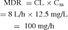
Thus the infusion rate should be 100 mg/h.
As the person’s condition improves, it is decided to switch to an oral dosing regimen, but it is essential to maintain the plasma drug concentration. The oral formulation has a bioavailability (F) of 0.8 (80%) and the recommended dosing interval is 8-hourly. Thus the oral maintenance dose can be calculated.
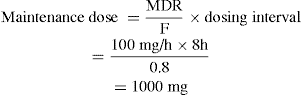
A formulation close to the ideal dose would then be prescribed. In this case drug D is available as a 500 mg capsule, so two capsules would be administered 8-hourly. If the drug were to be given 12-hourly, the dose would be 1500 mg (3 capsules).
Key pharmacokinetic concept—volume of distribution
It is important to understand that the term ‘volume of distribution’ is an abstract term and that it is not referring to a ‘real’ volume. For example, if a drug is tightly bound to plasma proteins, most of it will remain within the circulatory system and it will have a volume of distribution similar to that of the blood volume. If, however, it is distributed out of the circulatory system and binds to tissue proteins, less remains in the blood and the drug will appear to be distributed in a larger volume. The larger the volume, the more widespread (tissue-bound) the drug is within the body. This is illustrated in Figure 8-5 using a bucket filled to its maximum capacity of 5 L, which is its actual or real volume. When the drug remains in the ‘blood’ V remains at 5 L. However, when the drug distributes out of ‘blood’, even though it is still a 5 L bucket V becomes 50 L.
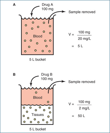
Figure 8-5 In this example the volume of the full bucket is 5 L and the amount of drug placed in each bucket is 100 mg. After the drug has distributed a ‘blood’ sample is removed from each bucket and the concentration of the drug measured. A Bucket A is filled with ‘blood’ to represent the circulatory system. Drug A binds tightly to plasma proteins and remains within the circulation. The concentration of drug measured in the ‘blood’ sample is 20 mg/L and the calculated volume of distribution of drug A is 5 L, the same as the volume of the bucket. B Bucket B is filled with a mixture of ‘blood’ and ‘tissues’ to represent the intravascular and extravascular compartments. Drug B moves from the ‘blood’ and is distributed to the ‘tissues’ where it binds strongly to tissue proteins. The concentration of drug measured in the ‘blood’ sample is 2 mg/L and the calculated volume of distribution of drug B is 50 L, 10 times greater than the volume of the bucket!
If the volume of distribution is ‘not a real volume’, of what use is it clinically? First, it provides an indication of accumulation of drugs in extravascular (tissue) compartments (e.g. fat, muscle). Second, it is a major determinant of the half-life of a drug (see the following
Box 8-4 Key pharmacokinetic definition: volume of distribution
The volume of distribution of a drug is defined as the volume in which the amount of drug in the body would need to be uniformly distributed to produce the observed concentration in the blood.
The volume of distribution of a drug (V) is calculated by dividing the total amount of drug in the body by the blood or plasma concentration of the drug.
section). Third, on occasion it is necessary to achieve a high plasma concentration quickly to produce the desired therapeutic response. To do this a loading dose is administered to ‘fill up’ the volume of distribution. The size of the loading dose is calculated by knowing the volume of distribution of the drug:

If we now consider drug D used in the maintenance dose calculation, the volume of distribution of drug D was known to be 40 L and the target plasma drug concentration was 12.5 mg/L.
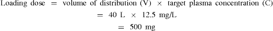
Thus the loading dose would be 500 mg. As rapid intravenous administration is often undesirable because of the high plasma concentrations achieved before the distribution phase, loading doses may be given over a period of minutes or even hours. In the example described above with drug D, the medical condition was acute and a loading dose (provided it was not contraindicated) could have been administered to produce a rapid pharmacological effect. Figure 8-2 shows that with the infusion alone it would take around 8 hours to achieve the desired plasma drug concentration (curve 2). In contrast, an IV bolus dose would raise the plasma drug concentration to the desired level almost immediately (Figure 8-2, curve 3).
The volume of distribution changes with age, body composition and disease states, and differs between males and females. For example in infants <1 year of age V is approximately 75%–80% of body weight; in adult males it is approximately 60% of body weight; and in adult females it is 55% of body weight. As we age there is also a progressive reduction in total body water and lean body mass with a relative increase in body fat. Some examples of volumes of distribution (normalised to a 70-kg person) are: warfarin, 8 L; frusemide, 12 L; theophylline, 35 L; digoxin, 420 L; cyclosporin, 1596 L; and fluoxetine, 2450 L.
Key pharmacokinetic concept—half-life
Use of the term half-life (t½) when referring to drugs is very common.
The half-life is the major determinant of:
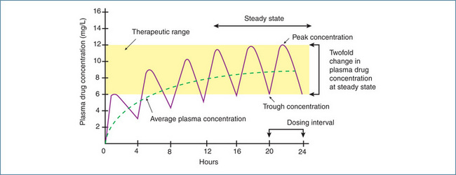
Figure 8-6 In this example, the drug has a half-life of 4 hours and is administered orally every 4 hours. After one half-life the average plasma concentration is 50% of the eventual steady-state concentration, which is reached after 3–5 half-lives. Once steady state is reached, the plasma drug concentration will fluctuate twofold between doses if dosing continues on the half-life.

Clinical interest Box 8-1 The dilemma of the missed dose
Often the question is raised ‘What do I do if I forget to take my medication?’ Inevitably, on one or more occasions, an individual will miss a dose of their drug. The simple issue of what to do if this occurs is rarely explained to patients, and an unintentionally missed dose is construed too readily as non-compliance. For some drugs (e.g. a lipid-lowering drug), a missed dose is of little consequence, but for others a missed dose can result in a decrease in the therapeutic plasma concentration and subsequent clinical manifestations (e.g. epilepsy). Pregnancy as a result of missing a dose of the oral contraceptive pill is well recognised.
Knowledge of the drug’s half-life is useful for making a recommendation if a dose is missed. In general when the clinical effect of a drug is related to its half-life, a single missed dose is less of a problem for a drug with a long half-life than for a drug with a short half-life, for which the therapeutic effect will be lost rapidly. For some drugs (e.g. the oral contraceptive pill), specific recommen dations exist for when a single dose is missed. A double dose should usually not be taken to make up for the dose missed because with many drugs (e.g. warfarin) this can cause adverse effects. The normal dosing regimen should be resumed and the next prescribed dose taken at the normal time (Gilbert et al 2002).
Factors influencing half-life
The two factors that influence half-life are volume of distribution and clearance. Changes in either of these pharmacokinetic parameters will alter the half-life of a drug. It can be seen from Figure 8-7 that, if two drugs have the same clearance but different volumes of distribution, the half-life is shorter for the drug with the smaller volume of distribution. Similarly, if the two drugs have the same volume of distribution but different clearances, the half-life is shorter for the drug with the higher clearance. This simple relationship explains why the half-life of a drug can change in individuals with heart failure because of decreased volume of distribution and decreased liver blood flow, and in persons with liver or kidney disease because of changes in clearance. Changes in half-life may necessitate changes in the dosing regimen.

Figure 8-7 Effects of volume of distribution and clearance on half-life. In A the drugs have the same clearance but differing volumes of distribution, and half-life differs about 10-fold. In B the drugs have the same volume of distribution but clearances differ about fourfold. In both examples the half-life alters in relation to the change in volume of distribution or the change in clearance.
Great importance is often placed on the half-life of a drug, but in fact it is a very poor indicator of the efficiency of drug elimination and, hence, the plasma drug concentration at steady state. For example, the half-life might be unaltered if both the volume of distribution of a drug and its clearance changed in the same direction. Under these circumstances, toxicity could occur if the usual maintenance dose rate were maintained (Clinical Interest Box 8-2).
Clinical interest Box 8-2 The danger of relying on half-life
This example illustrates how the half-life (t½) of a commonly prescribed drug called drug E can remain the same while the plasma drug concentration increases to toxic levels. The pharmacokinetic data (which are theoretical) for drug E have been obtained from standard drug information sources.

Unhealthy person with unstable physiology
In this person the volume of distribution and clearance for drug E have decreased.
This concentration is much higher than the upper limit of the therapeutic range (5 mg/L) and severe adverse reactions are highly likely. In this example, relying on the half-life is of no value. Clearly the dosing regimen should be changed.
Saturable metabolism
The last situation to consider is saturable metabolism, which is particularly relevant to some hepatic drugmetabolising enzymes. Anyone who has consumed alcohol to excess will have experienced the consequences of saturable hepatic metabolism. How often the comment is made that ‘It was the last drink that made me drunk’ and how true that is!
Our discussion of half-life assumed what is called first-order kinetics, that is, a constant proportion of the drug is eliminated per unit time. In that situation CL and t½ (assuming V does not change) are constant for a particular drug and the patient. As the dose and blood concentration of the drug increase, the rate of elimination also increases.
For example, elimination rate (mg/h) = CL (L/h) × C (mg/L). If CL is 10 L/h and the plasma drug concentration is 20 mg/L, the elimination rate is 200 mg/h. If C becomes 40 mg/L, the elimination rate becomes 400 mg/h.
Saturable metabolism is the situation in which the enzyme metabolising the particular drug reaches its maximum capacity and the rate of metabolism cannot increase further as the dose increases. This is called zero-order kinetics and in this situation the rate of elimination does not increase in proportion to the dose and concentration. At this stage, metabolism is said to be saturated and CL and t½ are no longer constant. CL continually decreases and t½ continually increases as the dose and blood concentration increase.
Using the example above, if a further dose of the drug is given increasing the plasma drug concentration to 80 mg/L but the rate of elimination is maximal (‘saturated’) at 400 mg/h, CL is reduced to 5 L/h. Characteristically a small change in dose can cause a large increase in the plasma drug concentration. This is illustrated in Figure 8-8 for the antiepileptic drug phenytoin. As a consequence of the zero-order kinetics, it is necessary to increase the phenytoin dose in small increments. Other drugs that exhibit saturable metabolism include salicylic acid and, of course, ethanol.
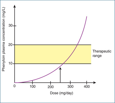
Figure 8-8 Illustration of the saturable metabolism of the antiepileptic drug phenytoin. Note that a small increment in dose above 250 mg/day results in a disproportionately large increase in phenytoin plasma concentration.
From the information presented in this chapter it is apparent that an understanding of basic pharmacokinetic principles is very important as this knowledge informs the clinical use of drugs and should allow for the rational design of dosing regimens.
Key points
 Rational use of drugs is based on the assumption that a particular concentration of a drug will have the desired therapeutic effect and that adverse effects will be negligible. For many drugs there is a sufficient relationship between plasma drug concentration and clinical response that dosing regimens are designed to maintain the concentration within a therapeutic range. The therapeutic range is generally considered to reflect the range of drug concentrations having a high probability of producing the desired therapeutic effect and a low probability of producing adverse effects. Pharmacokinetics plays a major role not only in establishing the initial dosing regimen but also in adjusting the regimen to deal with a lack of response or to reduce symptoms of toxicity. Clearance determines the maintenance dose rate required to achieve the target plasma concentration at steady state. The volume of distribution of a drug is defined as the volume in which the amount of drug in the body would need to be uniformly distributed in order to produce the observed concentration in blood.
Review exercises
References and further reading
Begg E.J. Instant Clinical Pharmacokinetics, 2nd edn. Oxford UK Wiley-Blackwell Publishing; 2007.
Birkett D.J. Pharmacokinetics Made Easy, 2nd edn. Sydney: McGraw-Hill; 2010.
Brody T.M., Larner J., Minneman K.P. Human Pharmacology: Molecular to Clinical, 3rd edn. St Louis: Mosby; 1998.
Gilbert A., Roughead L., Sansom L. I’ve missed a dose; what should I do? Australian Prescriber. 2002;25:16-18.
Holford N.H.G. Pharmacokinetics and pharmacodynamics: rational dosing and the time course of drug action. In Katzung B.G., editor: Basic and Clinical Pharmacology, 10th edn, New York: The McGraw-Hill Companies, 2007. [ch 3].
Rang H.P., Dale M.M., Ritter J.M., Flower R.J. Pharmacology, 6th edn. Edinburgh: Churchill Livingstone; 2007. [ch 8].
Rowland M., Tozer T.N. Clinical Pharmacokinetics Concepts and Applications, 3rd edn. Philadelphia: Lea & Febiger; 1995.
Somogyi A. Clinical pharmacokinetics and dosing schedules. In Brody T.M., Larner J., Minneman K.P., editors: Human Pharmacology: Molecular to Clinical, 3rd edn, St Louis: Mosby, 1998.