The ideal features of a dissolution apparatus are as follows:
1. The fabrication, dimensions and positioning of all components must be precisely specified and reproducible, run to run.
2. The apparatus must be simply designed, easy to operate and useable under a variety of conditions.
3. The apparatus must be sensitive enough to reveal process changes and formulation differences but still yield repeatable results under identical conditions.
4. In most cases, the apparatus should permit a controlled but variable intensity of mild, uniform, nonturbulent liquid agitation. Uniform flow is essential because changes in hydrodynamic flow will modify dissolution.
5. Nearly perfect sink conditions should be maintained.
6. The apparatus should provide an easy means of introducing the dosage form into the dissolution medium and holding it, once immersed, in a regular and reliable fashion.
7. The apparatus should provide minimum mechanical abrasion to the dosage form (with exceptions) during the test period to avoid disruption of the microenvironment surrounding the dissolving form.
8. Evaporation of the solvent medium must be eliminated and the medium must be maintained at a fixed temperature within a specified narrow range. Most apparati are thermostatically controlled at around 37°C.
9. Samples should be easily withdrawn for automatic or manual analysis without interrupting the flow characteristics of the liquid. In the latter case, efficient filtering should be achieved.
10. The apparatus should be capable of allowing the evaluation of disintegrating, nondisintegrating, dense or floating tablets or capsules and finely powdered drugs.
11. The apparatus should allow good interlaboratory agreement.
There are two principal types of apparatus design.
One is based on the limited volume that is constrained to the size of the container used. The second type uses a continuous flow cell to house the dosage form and permits constant replenishment of the dissolution fluids.
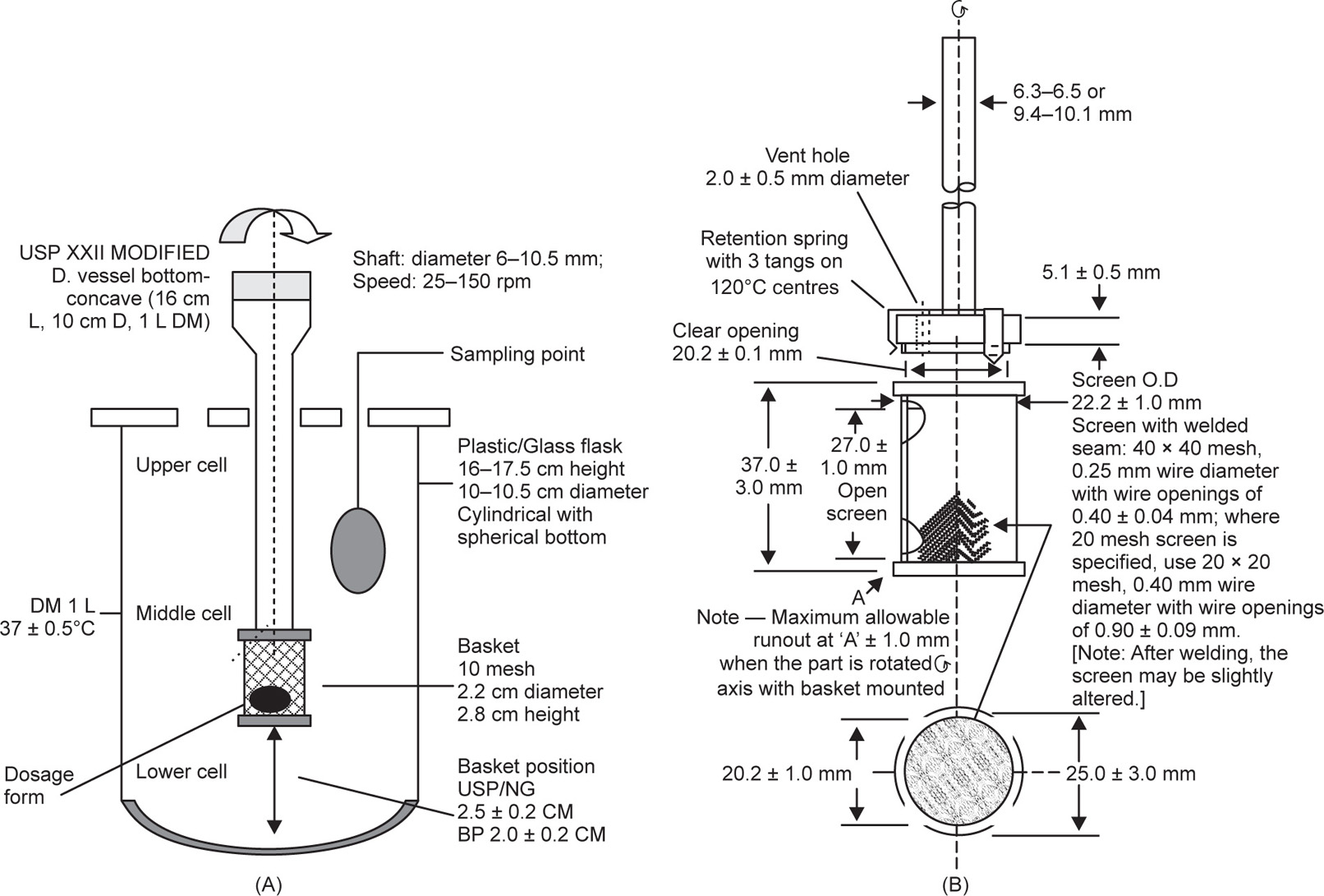
Basket Apparatus (USP Apparatus 1)
The basket method was first described in 1968 by Pernarowski et al. A container, the basket, constrained the enclosed tablet or capsule, allowed or fluid change and could be used either in continuous flow or in restricted volume modes. This gradually evolved to the USP XXVIII and BP 2004 Apparatus 1 – the Rotating Basket Apparatus (
Fig. 9.8). The dimensions are taken from the USP XXVIII, although those given in the BP 2004 are similar. The apparatus consists of a motor, a metallic drive shaft, a cylindrical basket and a covered vessel made of glass or other inert transparent material. The latter should be made of materials that do not sorb or react with the sample tested. The contents are held at 37 ± 0.5
oC. There should be no significant motion, agitation or vibration caused by anything other than the smoothly rotating stirring element. The vessel is cylindrical with a hemispherical bottom and sides that are flanged at the top. It is 160–175
mm high and has an inside diameter of 98–106
mm, and a nominal capacity of 1000
mL. A fitted cover may be used to retard evaporation but should provide sufficient openings to allow ready insertion of a thermometer and allow withdrawal of samples for analysis.
The shaft is so positioned that its axis is no more than 2mm at any point from the vertical axis of the vessel and should rotate smoothly, without significant wobble. The shaft rotation speed should be maintained within ±4% of the rate specified in the individual monograph. The shaft has a vent and three spring clips or other suitable means to fit the basket into position. Each should be fabricated of stainless steel, type 316 or equivalent. Welded seam and stainless steel cloth (40mesh or 425mm) is used, unless an alternative is specified. A 2.5mm thick gold coating on the basket may be used for acidic media. For testing, a dosage unit is placed in a dry basket at the beginning of each test. The distance between the inside bottom of the vessel and the basket is 25 ± 2mm. Although the basket apparatus in the USP XXVIII and BP 2004 are similar and have a common design, considerable changes have taken place since basket apparati were first included in official monographs.
The USP XVIII described a cylindrical vessel with a slightly concave bottom. The vessel was 16
cm high and has 10
cm internal diameter with a nominal capacity of 1000
mL. No precise specifications were given for the concave bottom, and differences in tolerances supplied by different manufacturers were common. Flask shape had affected the hydrodynamics of systems and consequently it was considered better to have flasks of uniform hemispherical shape. The flat-bottomed flask described in the BP 1980 alleviated the problems of manufacturing tolerances in vessel shape. Irrespective of apparatus design, there are still several potential problems. The wire basket corrodes following exposure to acidic media, the basket method gives poor reproducibility due to inhomogeneity of the agitation conditions produced by the rotating basket, and clogging of the basket can occur due to adhering substances. Additionally, particles can fall from
the rotating basket and sink to the bottom of the flask where they will not be subjected to the same agitation as that inside the basket. Finally, there is the possibility of dissolution being accelerated by abrasion of the dosage form’s surface as it rubs against the basket mesh—the so-called
cheese grater effect.
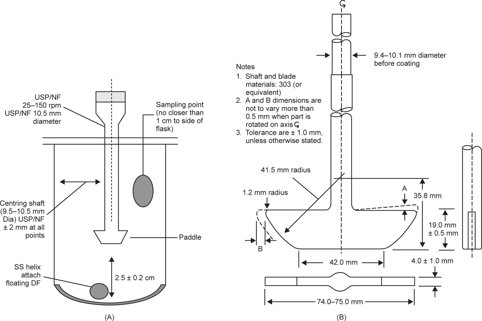
Paddle Apparatus (USP Apparatus 2)
An apparatus described by Levy and Hayes may be considered the forerunner of the beaker method. It consisted of a 400-mL beaker and a three-blade, centrally placed polyethylene stirrer (5
cm diameter) rotated at 59
rpm in 250
mL of dissolution fluid (0.1
N HCl). The tablet was placed down the side of the beaker and samples were removed periodically. In Apparatus 2, (
Fig. 9.9) the paddle apparatus method, a paddle replaces the basket as the source of agitation. As with the basket apparatus, the shaft should position no more than 2
mm at any point from the vertical axis of the vessel and rotate without significant wobble. The specifications of the shaft are given in
Fig. 9.9. A distance of 25 ± 2
mm between the blade and the inside bottom of the vessel is maintained during the test. The metallic blade and shaft comprise a single entity that may be coated with a suitable inert coating to prevent corrosion. The dosage form is allowed to sink to the bottom of the flask before rotation of the blade commences.
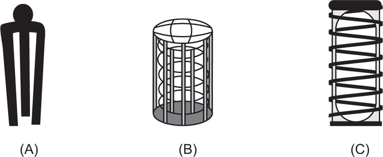
In the case of hard-gelatin capsules and other floating dosage forms, a ‘sinker’ is required to weight the sample down until it disintegrates and releases its contents at the bottom of the vessel. The sinker has to hold the capsule in a reproducible and stable position directly below the paddle, but it needs to be constructed in such a fashion that it does not significantly affect hydrodynamic flow within the vessel, nor should it appreciably reduce the surface area of the capsule available to the dissolution medium. Two designs have predominated, the three-fingered clip and the helical spring. The former comprises a small circular disc with three short, parallel rods sticking out from it, into which the capsule is wedged. The device is typically plastic but the disc contains metal, which gives it the necessary weight to fall to the bottom of the vessel. The latter is a stainless steel or plastic-coated stainless steel helix (coil, spring) down the middle of which is inserted the capsule. However, with this design, as the thickness of the wire used and the number of turns in the spring increase, the available surface area of the capsule decreases, leading to a concomitant decrease in the observed rate of dissolution.
The USP allows for ‘a small, loose piece of nonreactive material such as not more than a few turns of wire helix…’ while the Japanese Pharmacopoeia (JP) actually prescribes a specific sinker (
Fig. 9.10).
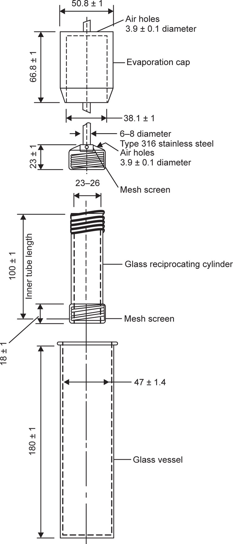
Flow-Through Cell Apparatus (USP Apparatus 4)
Limited-volume apparati with a finite volume of dissolution fluid suffer from the problem that they operate under nonsink conditions, which results in limitations when poorly soluble drugs are considered.
A flow-through system and reservoir may be used to provide sink conditions by continually removing solvent and replacing it with fresh solvent. Alternatively, continuous recirculation may be used when sink conditions are not required. The drawbacks of non-flow-through apparatus include (1) lack of flexibility, (2) lack of homogeneity, (3) the establishment of concentration gradients, (4) their semiquantitative agitation, (5) the obscuring of details of the dissolution processes and (6) their variable shear.
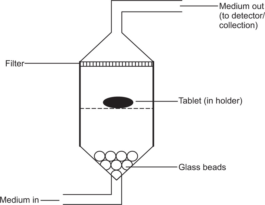
Consequently, the flow-through apparatus has been developed, which features a dissolution cell of low volume (often <30
mL) and a reservoir to provide fresh solvent. This is official in USP XXVIII as USP Apparatus 4 (
Fig. 9.12) where it is prescribed for testing extended-release articles.
The basic components are reservoir, pump, heat exchanger, column (cell), tablet support, filter system, and analytical method. The systems enable solvent to be taken from a suitable reservoir and passed straight through the apparatus containing the dosage form to be either assayed and removed (effluent system) or recirculated (recycling system). The design of the pump to remove the solvent from the reservoir is crucial to the results obtained from such systems. The pump used may be either a displacement (oscillating or peristaltic) or a momentum (centrifugal) type. However, peristaltic pumps may create oscillations that might result in faster dissolution rates than might otherwise have occurred.
Dissolution is affected by factors such as the volumetric flow rate, the cross-sectional area of the cell, the initial drug quantity, liquid velocity and drug concentration. The maintenance of a controlled flow is crucial to column methods and can be influenced by the inlet system. Laminar flow of solvent through the cell is achieved by placing glass beads at the bottom of the cell to facilitate similar disintegration of all surfaces of the sample. It is common to place the tablets on such supports, but attrition (by glass beads) may encourage breakdown of the dosage form thereby increasing dissolution rates. Tablet support and consistent positioning in the liquid flow are prerequisites for consistent results. Consequently, attempts have been made to embed the tablet in glass wool or glass beads. Laminar flow conditions are typically used for tablets, hard-gelatin capsules, powders and granules. Suppositories and soft-gelatin capsules are placed in the cell without beads for turbulent flow. Nicolaides, Hempenstall and Reppas have reported differences in the dissolution rate of a poorly soluble drug, tiaglitazone, from an immediate-release (IR) tablet formulation based on the presence or absence of a tablet holder and/or beads in the flow-through cell.
Flow-through facilities can be constructed from cylindrical chromatographic columns with flow rates as low as 1mL/min. Ascending flow minimizes the problems associated with air bubbles and allows laminar flow of the solvent and ascending columns are the most common types of flow-through apparatus. The columns may be short with tapered inlet and outlet sections but generally are long sections of straight-sided tubing to provide hydrodynamic stability to the liquid flow. The material under test is placed in the vertically mounted dissolution cell, which permits solvent at 37 ± 0.5°C to be pumped in from the bottom.
The cell type selected is dependent on the dosage form being tested. Standard cells used for tablets and capsules have an internal diameter of 12
mm but may show a higher dissolution rate when compared to 26
mm cells due to higher flow velocity. For testing powders and granules, a modified cell containing
two screen plates is used where the sample is placed between the screen plates. The suppository cell is designed for use with suppositories and soft gelatin capsules. Fats and gels used in these dosage forms are separated in this type of cell so as not to block the filters. The cell for implants has a 1
mL volume due to the low flow rates (e.g. 5
mL/h) required for testing this dosage form in a test that may continue over several weeks.
The flow rate of the dissolution medium through the cell must be specified for each product. The USP recommends a flow rate between 4 and 16mL/min with an allowance of ±5%. Manual operation and sampling for this type of test can be tedious and the system can be automated to control the pump, heat exchanger and test procedure, and deliver samples to a fraction collector. The system can be programmed to switch between different media at predetermined time points to allow pH changes during the test.
Further advantages of the flow through method include (1) selection of laminar or turbulent solvent flow conditions; (2) simple manipulation of medium pH to match physiological conditions; and (3) application to a wide range of dosage forms, e.g. tablets, hard and soft gelatin capsules, powders, granules, implants, and suppositories.
While the applicability of the flow-through apparatus to biorelevant dissolution tests still requires further investigation and optimization, an in vitro–in vivo correlation (IVIVC) has been reported with this apparatus using physiologically relevant flow rates and media.
Intrinsic Dissolution Method (USP)
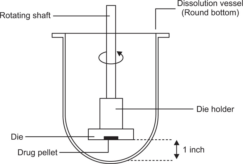
Two variations of the IDR apparatus exist—the rotating disc apparatus (Wood Apparatus,
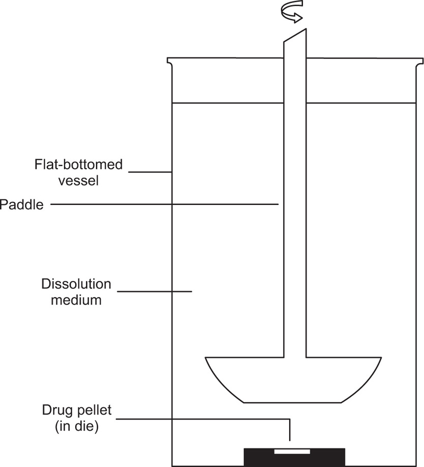
Fig. 9.13) and the stationary disc apparatus (
Fig. 9.14). Both types of apparatus employ a compacted pellet of pure drug produced by compressing an aliquot of powder in a stainless steel punch and die. The die is mounted onto a smooth polished-base plate and the punch is driven into the die using a hydraulic press. The USP states a compression dwell time of 1
min at the minimum compression force required to form a nondisintegrating compacted pellet. The
base plate is then detached to expose a smooth and constant pellet surface at the face of the die and it is this pellet surface that is subjected to the dissolution test. In the rotating disc apparatus, the die is then inverted and screwed onto a customized shaft on a dissolution tester, which is then lowered into the dissolution medium until the face pellet is 3.8
cm from the bottom of the vessel. The shaft is then rotated in the same way as USP Apparatus 1 and 2. In the stationary disc apparatus, the die containing compressed pellet is placed face up into a flat-bottomed dissolution vessel prefilled with the appropriate volume of dissolution medium. The medium is stirred by means of a rotating paddle (e.g. USP Apparatus 2) positioned 6
mm above the pellet surface.
Disadvantages of the rotating disk apparatus include the risk of air bubbles forming on the surface of the pellet, which could affect the dissolution rate and heat loss of approximately ±2oC through the shafts when the dies are first lowered into the dissolution medium. Using the stationary disc apparatus significantly reduces the formation of air bubbles, while heat losses are eliminated since the dies are totally submerged in the dissolution medium.
The IDR is calculated by plotting the cumulative amount of substance dissolved per unit area of the exposed pellet surface against time until 10% of the drug pellet has dissolved. Linear regression should be applied to data points up to this point and the slope of the regression line gives the IDR of the substance under test in mg/min/cm2. However, this compendia calculation may prove difficult to apply to poorly soluble compounds where 10% dissolution may not be achieved. In these instances, it may be practical to use an analytical method with sufficiently high sensitivity to be able to plot 6–8 data points before 10% dissolution and apply linear region.
 (9.1)
(9.1) (9.2)
(9.2)

 (9.3)
(9.3) (9.4)
(9.4)
 (9.5)
(9.5)

 (9.6)
(9.6)
 (9.7)
(9.7)
 (9.8)
(9.8) (9.9)
(9.9) (9.10)
 Cs, that is, sink condition, Eq. 9.10 simplifies to Eq. 9.11:
 (9.11)
 (9.12)
 (9.13)
 (9.14)
 (9.15)
 (9.16)
 (9.17)
 (9.18)
 (9.19)