Introduction

Sample statistics (such as , s) are estimates of the actual population parameters μ, σ. Even where adequate sampling procedures are adopted, there is no guarantee that the sample statistics are the exact representations of the true parameters of the population from which the samples were drawn. Therefore, inferences from sample statistics to population parameters necessarily involve the possibility of sampling error. As stated in Chapter 3, sampling errors represent the discrepancy between sample statistics and true population parameters. Given that investigators usually have no knowledge of the true population parameters, inferential statistics are employed to estimate the probable sampling errors. While sampling error cannot be completely eliminated, its probable magnitude can be calculated using inferential statistics. In this way investigators are in a position to calculate the probability of being accurate in their estimations of the actual population parameters.

The aims of this chapter are to examine how probability theory is applied to generating sampling distributions and how sampling distributions are used for estimating population parameters. Sampling distributions can be used for specifying confidence intervals, as discussed in this chapter, as well as for testing hypotheses, as further discussed in Chapter 18.

The specific aims of this chapter are to:

Probability

The concept of probability is central to the understanding of inferential statistics. Probability is expressed as a proportion between 0 and 1, where 0 means an event is certain not to occur, and 1 means an event is certain to occur. Therefore if the probability (p) is 0.01 for an event then it is unlikely to occur (chance is 1 in a hundred). If p = 0.99 then the event is highly likely to occur (chance is 99 in a hundred). The probability of any event (say event A) occurring is given by the formula:

Sometimes the probability of an event can be calculated a priori (before the event) by reasoning alone. For example, we can predict that the probability of throwing a head (H) with a fair coin is:

Or, if we buy a lottery ticket in a draw where there are 100 000 tickets, the probability of winning first prize is:

This is true only if the lottery is fair, if all tickets have an equal chance of being drawn by random selection.

In some situations, there is no model which we can apply to calculate the occurrence of an event a priori. For instance, how can we calculate the probability of an individual dying of a specific condition? In such instances, we use previously obtained empirical evidence to calculate probabilities a posteriori (after the event).

For example, if it is known that the percentages (or proportions) for causes of death are distributed in a particular way, then the probability of a particular cause of death for a given individual can be predicted. Table 17.1 represents a set of hypothetical statistics for a community.

Table 17.1 Causes of death for persons over 65

Given the data in Table 17.1, we are in a position to calculate the probability of a selected individual over 65 dying of any of the specified causes. For example, the probability of a given individual dying of coronary heart disease is:

This approach ignores individual risk factors and assumes that the environmental conditions under which the data were obtained are still pertinent. However, the example illustrates the principle that once we have organized the data into a frequency distribution we can calculate the probability of selecting any of the tabulated values. This is true whether the variable was measured on a nominal, ordinal, interval or ratio scale. Here, we will examine how to calculate the probability of values for normally distributed, continuous variables.

We can use the normal curve model, as outlined in Chapter 15, to determine the proportion or percentage of cases up to, or between, any specified scores. In this instance, probability is defined as the proportion of the total area cut off by the specified scores under the normal curve. The greater the proportion, the higher the probability of selecting the specified values.

For example, say that on the basis of previous evidence we can specify the frequency distribution of neonates’ weight. Let us assume that the distribution is approximately normal, with the mean () of 5.0 kg and a standard deviation (s) of 1.5. Now, say that we are interested in the probability of a randomly selected neonate having a birth weight of 2.0 kg or under. Figure 17.1 illustrates the above situation.

Figure 17.1 Frequency distribution of neonate birth weights. Area A1 corresponds to z ≤ –2.

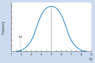
The area A1 under the curve in Figure 17.1 corresponds to the probability of obtaining a score of 2 or under. Using the principles outlined in Chapter 15 to calculate proportions or areas under the normal curve, we first translate the raw score of 2 into a z score:

Now we look up the area under the normal curve corresponding to z = − 2 (Appendix A). Here we find that A1 is 0.0228. This area corresponds to a probability, and we can say that ‘The probability of a neonate having a birth weight of 2 kg or less is 0.0228’. Another way of stating this outcome is that the chances are approximately 2 in 100, or 2%, for a child having such a birth weight.

We can also use the normal curve model to calculate the probability of selecting scores between any given values of a normally distributed continuous variable. For example, if we are interested in the probability of birth weights being between 6 and 8 kg, then this can be represented on the normal curve (area A2 on Fig. 17.2). To determine this area, we proceed as outlined in Chapter 15. Let s = 1.5.

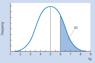
Figure 17.2 Frequency distribution of neonate birth weights. Area A2 corresponds to probability of weight being 6–8 kg.

Therefore: the area between z₁ and is 0.2486 (from Appendix A) and the area between z₂ and = 0.4772 (from Appendix A). Therefore, the required area A2 is:

It can be concluded that the probability of a randomly selected child having a birth weight between 6 and 8 kg is p = 0.2286. Another way of saying this is that there is a chance of 23 in 100 or a 23% chance that the birth weight will be between 6 and 8 kg.

The above examples demonstrate that when the mean and standard deviation are known for a normally distributed continuous variable, this information can be applied to calculating the probability of events related to this distribution. Of course, probabilities can be calculated for other than normal data but this requires integral calculus which is beyond the scope of this text. In general, regardless of the shape or scaling of a distribution, scores which are common or ‘average’ are more likely to be selected than those which are atypical, being unusually high or low.

Sampling distributions

Probability theory can also be applied to calculate the probability of obtaining specific samples from populations.

Consider a container with a very large number of identically sized marbles. Imagine that there are two kinds of marbles present, black (B) and white (W), and that these colours are present in equal proportions, so that p (B) =p (W) = 0.5.

Given the above population, say that samples of marbles are drawn randomly and with replacement. (By ‘replacement’ we mean the samples are put back into the population, in order to maintain as a constant the proportion of B = W = 0.5.) If we draw samples of four (that is, n = 4) then the possible proportions of black and white marbles in the samples can be deduced a priori as shown in Figure 17.3.

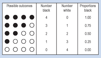
Figure 17.3 Characteristics of possible samples of n = 4, drawn from a population of black and white marbles.

Ignoring the order in which marbles are chosen, Figure 17.3 demonstrates all the possible outcomes for the composition of samples of n = 4. It is logically possible to draw any of the samples shown. However, only one of the samples (2B, 2W), is representative of the true population parameter. The other samples would generate incorrect inferences concerning the state of the population. In general, if we know or assume (hypothesize) the true population parameters, we can generate distributions of the probability of obtaining samples of a given characteristic.

In this instance, when attempting to predict the probability of specific samples drawn from a population with two discrete elements, the binomial theorem can be applied. The expansion of the binomial expression, (P + Q)ⁿ, generates the probability of all the possible samples which can be drawn from a given population. The general equation for expanding the binomial expression is:

P is the probability of the first outcome, Q is the probability of the second outcome and n is the number of trials (or the sample size).

In this instance, P =proportion black (B) = 0.5; Q = proportion white (W) = 0.5; n = 4 (sample size). Therefore, substituting into the binomial expression:

Note that each part of the expansion stands for a probability of obtaining a specific sample. For the present case:

The calculated probabilities add up to 1, indicating that all the possible sample outcomes have been accounted for. However, the important issue here is not so much the mathematical details but the general principle being illustrated by the example. For a given sample size (n) we can employ a mathematical formula to calculate the probability of obtaining all the possible samples from a population with known parameters. The relationship between the possible samples and their probabilities can be graphed, as shown in Figure 17.4.

Figure 17.4 Sampling distribution of black marbles; n = 4.

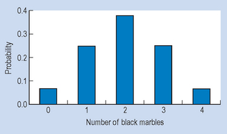
Taking the statistic ‘number of black marbles in the sample’, the graph in Figure 17.4 shows the probability of obtaining any of the outcomes. The distribution shown is called a ‘sampling distribution’. In general, a sampling distribution for a statistic indicates the probability of obtaining any of the possible values of a statistic.

Therefore, having obtained our sampling distribution we can see that some sample outcomes have low probability while others are more likely. Although there is a finite chance of obtaining a sample such as ‘all blacks’, the probability of this happening is rather small (p = 0.0625). Conversely, a sample of 2B2W, which is equal to the true population proportions, is far more probable (p = 0.375). Generating sampling distributions for calculating the probability of given sample statistics is a basic practice in inferential statistics. The sampling distributions enable researchers to infer (with a determined level of confidence) the true population parameters from the sample statistics.

Sampling distribution of the mean

The binomial theorem is appropriate for generating sampling distributions for discontinuous nominal scale data. However, when measurements are continuous, the mean and standard deviations are appropriate as sample statistics and are measured on interval or ratio scales. The sampling distribution of the mean represents the frequency distribution of sample means obtained from random samples drawn from the population. The sampling distribution of the mean enables the calculation of the probability of obtaining any given sample mean (). This is essential for testing hypotheses about sample means (Ch. 18).

In order to generate the sampling distribution of the mean, we use a mathematical theorem called the central limit theorem. This theorem provides a set of rules which relate the parameters (μ, σ) of the population from which samples are drawn to the distribution of sample means ().

The central limit theorem states that if random samples of a fixed n are drawn from any population, as n becomes large the distribution of sample means approaches a normal distribution, with the mean of the sample means ( or μ) being equal to the population mean (μ) and the standard error of estimate (s or σ) being equal to σ/. The standard error of the estimate is the standard deviation of the distribution of sample means.

Let us follow the above step by step.

3. Having obtained our samples, for each sample we calculate the sample mean (₁, ₂, … and so on).

4. Each sample mean, , is a number. The sampling distribution of the mean is a frequency distribution representing the large number of sample means.

5. The central limit theorem predicts theoretically the shape (normal for large n), mean ( or μ) and standard deviation (s or σ) of a large number of sample means.

It should be noted that:

2. The mean of the sample means (μ or ) is the mean of the distribution of sample means. and μ are equal to μ, the population mean.

3. The standard error of the mean (s or σ) is the standard deviation of the frequency distribution of sample means drawn from a population. The magnitude of s or σ is equal to σ/, the population standard deviation divided by the square root of the sample size.

4. μ and σ are used in reference to a sampling distribution based on all the possible samples drawn from a population (a population of samples, would you believe?), while and s are used when the sampling distribution is based on a ‘sample’ of samples.

Let us have a look at an example. Assume for a hypothetical test of motor function that μ= 50 and σ= 10. What is the probability of drawing a random sample from this population with = 52 or greater (i.e. ≥ 52) given that n = 100? The central limit theorem predicts that when we draw samples of n = 100 from the above population, the sampling distribution of the means will be as follows:

• The standard error of estimate (σ) will be:

(We can show this as in Fig. 17.5.)

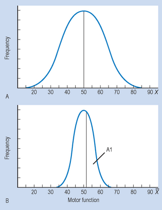
Figure 17.5 Relationship between original population and sampling distribution of the mean, where μ= 50 and σ= 10; (A) original population, (B) sampling distribution of the mean.

Previously, we saw how we can use normal frequency distributions for estimating probabilities. Using the same principles as in Chapter 15, we can calculate the z score corresponding to = 52, and look up Appendix A to find out the area representing the probability in question:

That is, = 52 is two standard error units above μ, the population mean for the sample means.

You may have noticed that the distribution of is far less dispersed than X (i.e. the raw scores), as σ= 1 and σ= 10.

Using Appendix A for establishing the probability, we find that the area representing p ( ≥ 52), that is, area A1 in Figure 17.5B, is:

Therefore the probability of drawing a sample of ≥ 52 is 0.0228. We will apply this notion to hypothesis testing in Chapter 18, but you might have noticed that it is a rather low probability. That is, it is unlikely (p = 0.0228) randomly to draw a sample with ≥ 52 where n = 100 and μ= 50.

Application of the central limit theorem to calculating confidence intervals

Let us assume that you are asked to estimate the weight of a newborn baby. If you are experienced in working with neonates, you should be able to make a reasonable guess. You might say ‘The baby is 6 kg’. Someone might ask ‘How certain are you that the baby is exactly 6 kg?’ You might then say ‘Well, the baby might not be exactly 6 kg, but I’m very confident that it weighs somewhere between 5.5 and 6.5 kg’. This statement expresses a confidence interval – a range of values which probably include the true value. Of course, the more certain or confident you want to be of including the true value, the bigger the range of values you might give: you are unlikely to be wrong if you guess that the baby weighs between 4 and 8 kg.

Confidence intervals can be calculated for a large range of statistics such as proportions, ratios or correlation coefficients. In this chapter we will look at confidence intervals for single samples as an illustration for using confidence intervals.

We have seen previously that if we know the population parameters we can estimate the probability of selecting from that population a sample mean of a given magnitude. Conversely, if we know the sample mean we can estimate the population parameters from which the sample might have come, at a given level of probability. Let us take an example to illustrate this point.

A researcher is interested in the systolic blood pressure (BP) levels of smokers of more than 10 cigarettes per day. She takes a random sample of 100 10+ smokers in her district and finds that the mean BP = 148 mmHg for the sample, with a standard deviation of s = 10.

She wants to generalize to the population of smokers of more than 10 cigarettes per day in their district. The best estimate of μ (the population parameter) is 148, but it is possible that, because of sampling error, 148 is not the exact population parameter. However she can calculate a confidence interval (a range of blood pressures that will include the true population mean at a given level of probability). A confidence interval is a range of scores which includes the true population parameter at a specified level of probability. The precise probability is decided by the researcher and indicates how certain she can be that the population mean is actually within the calculated range. Common confidence intervals used in statistics are 95% confidence intervals, which offer a probability of p = 0.95 for including the true population mean, and 99% confidence intervals, which include the true population mean at a probability of p = 0.99.

Calculating the confidence interval requires the use of the following formula:

where is the sample mean; z is the z score obtained from the normal curve table such that it cuts off the area of the normal curve corresponding to the required probability; s is the sample standard error, which is equal to the sample standard deviation divided by √n, that is, s = s/√n.

Let us turn to the previous example to illustrate the use of the above equation. Here = 148, and s = 51/√100. Assume that we want to calculate a 95% confidence interval. We are looking for a pair of z scores which have 95% of the standard normal curve between them. In this case, 1.96 is the value for z which cuts off 95% of a normal distribution. That is, we looked up the value of z corresponding to an area (probability) of 0.4750, since the 0.05 has to be divided among the two tails of the distribution, giving 0.025 at either end. Substituting into the equation above we have:

That is, the investigator is 95% confident that the true population mean, the true mean BP of smokers, lies between 146.04 (lower limit) and 149.96 (upper limit). There is only a 5% or 0.05 probability that it lies outside this range. If we chose a 99% confidence interval, then using the formula as above, we have:

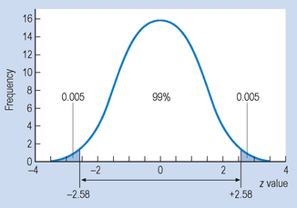
Here, 2.58 is the value of z which cuts off 99% of a normal distribution (Fig. 17.6). That is, the investigator is 99% confident that the true population mean lies somewhere between 145.42 and 150.58. Clearly, the 99% interval is wider than the 95% interval; after all, here the probability of including the true mean is greater than for the 95% interval. Conventionally, health sciences publications report 95% confidence intervals.

Figure 17.6 z scores for 99% confidence interval.

Confidence intervals where n is small: the t distribution

It was previously stated that: ‘as n becomes large, the distribution of sample means approaches a normal distribution’ (central limit theorem). The questions left to explain are:

It has been shown by mathematicians that the sample size, n, for which the sampling distribution of the mean can be considered an approximation of a normal distribution is n ≥ 30. That is, if n is 30 or more, we can use the standard normal curve to describe the sampling distribution of the mean. However, when n < 30, the sampling distribution of the mean is a rather rough approximation to the normal distribution. Instead of using the normal distribution, we use the t distribution, which takes into account the variability of the shape of the sampling distribution due to low n.

The t distributions (Fig. 17.7) are a family of curves representing the sampling distributions of means drawn from a population when sample size, n, is small (n < 30). A ‘family of curves’ means that the shape of the t distribution varies with sample size. It has been found that the distribution is determined by the degrees of freedom of the statistic.

Figure 17.7 t distributions.

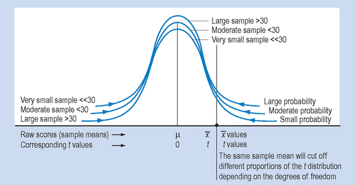
The degrees of freedom (df) for a statistic represents the number of scores which are free to vary when calculating the statistic. Since the statistic we are calculating in this case is the mean, all but one of the scores could vary. That is, if you were inventing scores in a sample with a known mean, you would have a free hand until the very last score. There df is equal to n − 1 (the sample size minus one). Each row of figures shown in Appendix B represents the critical values of t for a given distribution.

The t distribution, just as the z distribution, can be used to approximate the probability of drawing sample means of a given magnitude from a population; t can also be used for calculating confidence intervals. Let us re-examine the example relating to the blood pressure of smokers presented earlier. Let us assume that n = 25, with the other statistics remaining the same: = 148, s = 10. The general formula for calculating the confidence intervals for small samples is:

You will note the similarity to the equation on page 199; here t replaces z. If we want to show the 95% confidence interval, then we use the same logic as for z distributions (Fig. 17.8).

Figure 17.8 The 95% confidence interval for sample size of 25.

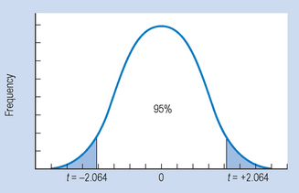
To look up the t values from the tables (Appendix B) consider (i) direction, (ii) probabilities and (iii) degrees of freedom.

We are looking at a ‘non-directional’ or ‘two-tail’ probability in the sense that the t values cut off 95% of the area of the t curve between them, leaving 5% distributed at the two tails of the t distribution: p = 0.05; df = 25 − 1 = 24. Therefore t = 2.064 (from Appendix B). Substituting into the equation for calculating confidence intervals:

Consider the width of the confidence interval defined as the distance between the upper and lower limits. Note that this is a wider interval than that which was obtained when n was 100. As sample size, n, becomes smaller, our confidence interval becomes wider, reflecting a greater probability of sampling error.

To calculate the 99% confidence interval (Fig. 17.9) we need to look up p = 0.01, nondirectional, df = 24 in Appendix B to obtain the critical value of t, which is 2.797.

Figure 17.9 The 99% confidence interval for sample size of 25.

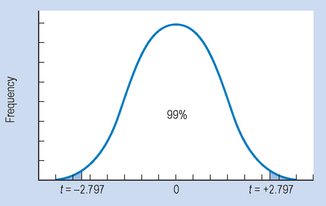
We can see that, when n = 25, the 99% confidence interval is wider than for n = 100. That is, the bigger our sample size, the narrower (more precise) our estimate of the range of values (which includes the true population parameter) becomes when our sample size is large.

Summary

It was argued in this chapter that, even with randomly selected samples, the possibility of sampling error must be taken into account when making inferences from sample statistics to population parameters. It was shown that probability theory can be applied to generating sampling distributions, which express the probability of obtaining a given sample from a population. With discontinuous, nominal data the binomial theorem provides an adequate mathematical distribution for estimating the probability of obtaining possible samples. However, with continuous data, the central limit theorem is applied to generate the sampling distributions of the mean. The standard distribution of the mean enables the calculation of the probability-specified sample mean(s) by random selection. The sampling error of the mean (s or σ), which expresses statistically the range of the sampling error, depends inversely on the sample size, such that the larger the n, the smaller the s or σ.

One of the applications of sampling distributions is for calculating confidence intervals for continuous data. Confidence intervals represent a range of scores which specify, from sample data, the probability of capturing the true population parameters.

Health researchers usually report 95% confidence intervals. When sample sizes are small (n < 30), the t distribution is appropriate for representing the sampling distribution of the mean. With large sample sizes, the two distributions merge together. As the next chapter will demonstrate, sampling distributions are essential for testing hypotheses, a procedure which uses inferential statistics to calculate the level of probability at which sample statistics support the predictions of hypotheses.

Self-assessment

Explain the meaning of the following terms:

True or false

1. If death and taxes are an absolute certainty, then the probability of their occurrence is infinite.

2. Probability values fall between 0 and 1.

3. When a score occurs at a relatively high level of frequency the probability of randomly selecting it from a distribution is p = 1.

4. The higher the corresponding z score, the lower the probability of randomly selecting the score from a distribution.

5. For a normal distribution, σ is the score which has the highest probability of random selection.

6. It is possible to have a negative z score but not a negative probability.

7. For a continuous normal distribution, the probability of selecting a score up to and including the mode is p = 0.5.

8. The probability of randomly selecting a score 2 standard deviations above the mean is p = 0.2.

9. We can generate appropriate sampling distributions for statistics derived from nominal or ordinal data.

10. Statistical inference involves the estimation of population parameters from sample statistics.

11. Statistical inference depends on knowing the true population parameters before beginning research.

12. The sampling distribution of the mean is a frequency polygon of mean scores.

13. Using the sample mean as an estimate for the population mean is an example of statistical inference.

  Page 203 

14. The sampling distribution of the mean is always normally distributed.

15. As n increases, the variability of the sampling distribution of the mean increases.

16. μ = μ regardless of the shape of the sampling distribution of the mean.

17. The characteristics of the sampling distribution of the mean vary with the size of the sample.

18. If a random selection method is used, sampling error will be zero.

19. The bigger the sampling error, the smaller the confidence interval.

20. Generally speaking, the higher the level of confidence we have that an interval contains the population mean, the larger is that interval.

Multiple choice

1. The mean age of the Canadian population is known to be 31 years. A small randomly selected sample of Canadians is found to have a mean age of 32. This discrepancy is an example of:

a a sampling error

b a measurement error

c a problem in ecological validity

d failure to control for the effects of maturation.

At a large maternity hospital the following hypothetical data are compiled concerning the birth weights and survival of neonates.

Weight of neonates (g)	Numbers (n)	Percentage of neonates surviving
0–499	25	40
500–999	50	60
1000–1499	75	80
1500–1999	150	90
2000–2499	250	95
2500	450	98

Questions 2–5 refer to this table.

2. What is the probability that a randomly selected neonate will weigh under 500 g?

a 0.4000

b 0.1700

c 0.0250

d 0.0025

3. What is the probability that a randomly selected neonate will have a birth weight of 2000 g or over?

a 0.7000

b 0.9638

c 0.3000

d 0.9500

4. What is the probability that a neonate weighing 499 g or under will survive?

a 0.4000

b 0.1700

c 0.040

d 0.025

5. What is the probability that a neonate weighing 2500 g or over will not survive?

a 0.400

b 0.300

c 0.006

d 0.020

A test of reaction times has a mean of 10 and a standard deviation of 4 in the normal adult population with a normal distribution. Questions 6–12 refer to this information.

6. A person scores 8. That person’s z score is:

a 2

b − 2

c − 0.5

d − 1

7. What percentage of the population would have scores up to and including 14 on this test?

a 84.13

b 15.87

c 65.87

d 34.13

8. What is the percentile rank of a score of 8 on this test?

a 19.15

b 30.85

c 80.85

d 53.28

9. What score (to the nearest whole number) would cut off the highest 10% of scores?

a 1

b 14

  Page 204 

c 15

d 18

10. What is the probability that a randomly selected individual will score greater than 6 on this test?

a 0.4987

b 0.3413

c 0.8413

d 0.6587

11. What is the probability that a randomly selected individual will score between 8 and 14 on this test?

a 0.1498

b 0.5328

c 0.6816

d 0.4671

12. What is the probability that a randomly selected individual will score either more than 14 or less than 10 on this test?

a 0.6587

b 0.6816

c 0.3184

d 0.8184

13. Sampling error of the mean:

a occurs because of poor sampling techniques

b decreases as sample size increases

c is independent of the standard deviation

d is always equal to 1.

14. Samples of 100 are drawn from a normally distributed population with a mean of 50 and a standard deviation of 10. The distribution of sample means will:

a have a mean of 50

b have a standard deviation of 1

c be normally distributed

d all of the above.

15. Increasing the sample size, n :

a decreases sampling error

b increases sampling error

c has no effect on standard error of the mean

d requires increasing correction of sample estimates of population parameters

e none of these.

16. If the dispersion of the raw score population increases while n is held constant, σ:

a decreases

b increases

c remains the same

d cannot be ascertained without more information.

17. The sampling distribution of the mean:

a is always positively skewed for continuous data

b is normally distributed if the population raw scores are not normally distributed

c is approximately normally distributed if sample size is large

d all of the above.

18. As the degrees of freedom decrease, the similarity between the t and z distributions:

a increases

b decreases

c remains the same

d approaches infinity.

19. The theoretical sampling distributions of the t statistics depend on:

a p

b r

c s

d df.

A normally distributed population has a mean of 80 and a standard deviation of 12. Questions 20–24 refer to this information.

20. For samples of n = 36, what is the standard error of the mean?

a 12

b 0.33

c 2

d 3

21. A sample of 64 cases is found to have a mean of 83. What is the z score of this mean?

a 2

b 0.25

c 4

d 1.5

22. A sample of n = 144 has a mean of 77. What is the probability that a mean this low would occur by chance?

a 0.0300

b 0.0013

c 0.4989

d 0.9987

23. A sample of 36 cases is selected. What is the probability that its mean falls outside the range of 79–81?

a 0.6813

b 0.8085

c 0.3085

d 0.6170

  Page 205 

24. Which is more likely: that a randomly selected sample of n = 36 will have a mean greater than 82 or that it will have a mean less than 77?

a Greater than 82.

b Less than 77.

c Both are equally probable.

d Impossible to tell.

25. The t distribution differs from the z distribution in which of these ways?

a Its mean is not exactly equal to 0.

b It is not quite symmetrical.

c It is somewhat wider and flatter.

d All of the above.

26. The 95% confidence interval arrived at from a particular experiment is 72–79. Therefore:

a the probability is 0.05 that μ falls between 72–79

b the probability is 0.95 that the interval 72–79 contains

c the probability is 0.95 that the interval 72–79 contains μ

d a and c.

27. Compared with a 99% confidence interval, a 95% confidence interval is:

a larger

b smaller

c more likely to contain the population mean

d less likely to contain the sample mean.

The following information should be used in answering questions 28–31: a random sample of 25 clients is selected, and their systolic blood pressures measured; the mean BP is 115 mmHg, with a standard deviation of 10.

28. This is an example of:

a an experiment

b a natural comparison study

c a survey

d field research.

29. What is the standard error of the mean for a sample of this size?

a 10

b 20

c 2

d 2.5

30. In order to calculate the 99% confidence interval of the mean, what t score will be used?

a 2.492

b 2.787

c 2.797

d 1.711

31. What is the 99% confidence interval of the mean in this example?

a 110.0 ≤ μ ≤ 120.0

b 109.4 ≤ μ ≤ 120.6

c 111.6 ≤ μ ≤ 118.4

d 113.0 ≤ μ ≤ 117.0

32. A random sample of 25 university students is found to have a mean IQ of 110, with a standard deviation of 10. Between what two possible scores can we be 99% confident that the true mean IQ for the students at the university lies?

a 95.5–112.5

b 85–135

c 102.4–117.6

d 104.1–115.9

In order to establish the mean weight of newborn babies at a large maternity hospital, a random sample of 64 babies is weighed. Their mean weight is 2500 g, with a standard deviation of 80 g.

Questions 33–35 refer to this information.

33. What is the standard error of the mean?

a 80

b 10

c 1.25

d 0.1

34. In calculating the 95% confidence interval of the mean, what z value is used?

a 1.96

b 2.33

c 2.58

d 1.64

35. What is the 95% confidence interval of the mean in this example (to the nearest whole number)?

a 2480 ≤ μ ≤ 2520

b 2477 ≤ μ ≤ 2523

c 2474 ≤ μ ≤ 2526

d 2484 ≤ μ ≤ 2516

  Page 206