Introduction

In the previous chapter we introduced the use of inferential statistics for estimating population parameters from sample statistics. In the case of some non-experimental research projects, such as surveys and descriptive statistics, parameter estimation is adequate for analysing the data. After all, these investigations aim at describing the characteristics of specific populations. However, other research strategies involve data collection for the purpose of testing hypotheses. Here the investigator has to establish if the data support or refute the hypotheses being investigated. The key issue is that hypotheses are generalizations addressing differences in patterns and associations in populations. Inferential statistics enables us to calculate the probability (level of significance) for asserting that what we are seeing in our sample data is generalizable to the population. This probability is related to the statistical significance of the sample data.

The aim of this chapter is to introduce the logical steps involved in hypothesis testing in quantitative research. Given that hypothesis testing is probabilistic, special attention must be paid to the possibility of making erroneous decisions, and to the implications of making such errors.

The specific aims of the chapter are to:

A simple illustration of hypothesis testing

One of the simplest forms of gambling is betting on the fall of a coin. Let us play a little game. We, the authors, will toss a coin. If it comes out heads (H) you will give us £1; if tails (T) we will give you £1. To make things interesting, let us have 10 tosses. The results are:

Oh dear, you seem to have lost. Never mind, we were just lucky, so send along your cheque for £10. What is that, you are a little hesitant? Are you saying that we ‘fixed’ the game? There is a systematic procedure for demonstrating the probable truth of your allegations:

The probability of calculating the truth of H₀ depended on the number of tosses (n = the sample size). For instance, the probabilities of obtaining all heads with up to five tosses, according to the binomial theorem (Ch. 17), are shown in Table 18.1. The table shows that, as the sample size (n) becomes larger, the probability at which it is possible to reject H₀ becomes smaller. With only a few tosses we really cannot be sure if the game is fixed or not: without sufficient information it becomes hard to reject H₀ at a reasonable level of probability.

Table 18.1 Probability of obtaining all heads in coin tosses

A question emerges: ‘What is a reasonable level of probability for rejecting H₀?’ As we shall see, there are conventions for specifying these probabilities. One way to proceed, however, is to set the appropriate probability for rejecting H₀ on the basis of the implications of erroneous decisions.

Obviously, any decision made on a probabilistic basis might be erroneous. Two types of elementary decision errors are identified in statistics as Type I and Type II errors. A Type I error involves mistakenly rejecting H₀, while a Type II error involves mistakenly retaining H₀.

In the above example, a Type I error would involve deciding that the outcome was not due to chance when in fact it was. The practical outcome of this would be to accuse the authors falsely of fixing the game. A Type II error would represent the decision that the outcome was due to chance, when in fact it was due to a ‘fix’. The practical outcome of this would be to send your hard-earned £10 to a couple of crooks. Clearly, in a situation like this, a Type II error would be more odious than a Type I error, and you would set a fairly high probability for rejecting H₀. However, if you were gambling with a villain, who had a loaded revolver handy, you would tend to set a very low probability for rejecting H₀. We will examine these ideas more formally in subsequent parts of this chapter.

The logic of hypothesis testing

Hypothesis testing is the process of deciding statistically whether the findings of an investigation reflect chance or real effects at a given level of probability. If the results do not represent chance effects then we say that the results are statistically significant. That is, when we say that our results are statistically significant we mean that the patterns or differences seen in the sample data are generalizable to the population.

The mathematical procedures for hypothesis testing are based on the application of probability theory and sampling, as discussed previously. Because of the probabilistic nature of the process, decision errors in hypothesis testing cannot be entirely eliminated. However, the procedures outlined in this section enable us to specify the probability level at which we can claim that the data obtained in an investigation support experimental hypotheses. This procedure is fundamental for determining the statistical significance of the data as well as being relevant to the logic of clinical decision making.

Steps in hypothesis testing

The following steps are conventionally followed in hypothesis testing:

Let us look at an example. A rehabilitation therapist devises an exercise programme which is expected to reduce the time taken for people to leave hospital following orthopaedic surgery. Previous records show that the recovery time for patients has been μ = 30 days, with σ = 8 days. A sample of 64 patients are treated with the exercise programme, and their mean recovery time is found to be = 24 days. Do these results show that patients who had the treatment recovered significantly faster than previous patients? We can apply the steps for hypothesis testing to make our decision.

2. State H₀: ‘The exercise programme does not reduce the time taken for patients to recover from orthopaedic surgery’. That is, the statement claims that the independent variable has no effect on the dependent variable. The statement implies that the treated sample with = 24, and n = 64 is in fact a random sample from the population μ = 30, σ = 8. Any difference between and μ can be attributed to sampling error.

4. Calculate the probability of H₀ being true. As stated above, H₀ implies that the sample with = 24 is a random sample from the population with μ = 30, σ = 8. How probable is it that this statement is true? To calculate this probability, we must generate an appropriate sampling distribution. As we have seen in Chapter 17, the sampling distribution of the mean will enable us to calculate the probability of obtaining a sample mean of = 24 or more extreme from a population with known parameters. As shown in Figure 18.1, we can calculate the probability of drawing a sample mean of = 24 or less. Using the table of normal curves (Appendix A), as outlined previously, we find that the probability of randomly selecting a sample mean of = 24 (or less) is extremely small. In terms of our table, which only shows the exact probability of up to z = 4.00, we can see that the present probability is less than 0.00003. Therefore, the probability that H₀ is true is less than 0.00003.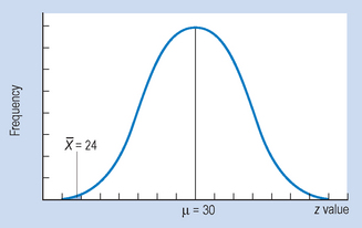

Figure 18.1 Sampling distribution of means. Sample size = 64; population mean = 30; standard deviation = 8.

Directional and non-directional hypotheses and corresponding critical values of statistics

In the previous example, H_A was directional in that we asserted that the difference between the mean of the treated sample and the population mean was expected to be in a particular direction. If we state that there was some effect due to the dependent variable, but do not specify which way, then H_A is called non-directional. In the previous example, if the investigator stated H_A as ‘The exercise programme changes the time taken to recover following surgery’ then H_A would have been non-directional.

In general, an alternative hypothesis is directional if it predicts a specific outcome concerning the direction of the findings by stating that one group mean will be higher or lower than the other(s). An alternative hypothesis is non-directional if it predicts a difference, without specifying which group mean is expected to be higher or lower than the others.

If we propose a directional H_A, it is understood that we have reasonable information on the basis of pilot studies or previously published research for predicting the direction of the outcome. The advantage of a directional H_A is that it increases the probability of rejecting H₀. However, the decision of the directionality of H_A must be decided before the data are collected and analysed.

Let us now examine the concept of the ‘critical’ value of a statistic. The critical value of a statistic is the value of the statistic which bounds the proportion of the sampling distribution specified by α. The critical value of the statistic is influenced by whether H_A is directional or non-directional.

Figures 18.2 and 18.3 represent the sampling distributions of the mean where n is large; that is, the sampling distribution for the statistic .

Figure 18.2 Two examples of statistical decision making with directional (one-tail) hypothesis, H_A.

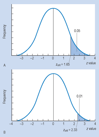
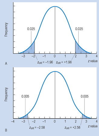
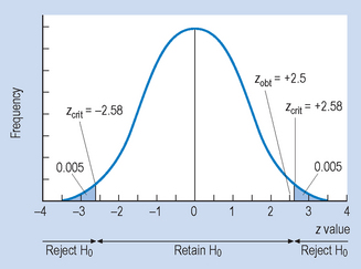
Figure 18.3 Two examples of statistical decision making with non-directional (two-tail) hypothesis, H_A.

As we have seen in Chapter 17, these are the sampling distributions for we would expect by the random selection of samples, as specified by H₀. Therefore, we can estimate from the distributions the probability of selecting any sample mean, , by chance alone. The α value (the level of significance) specifies the criterion for rejecting H₀. We can see that the critical value for the statistic (in this case z_crit) cuts off an area of the distribution corresponding to α (p = 0.05 or p = 0.01).

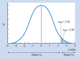
In Figure 18.2, we can see that z_crit = 1.65 (for α = 0.05) and z_crit = 2.33 (for α = 0.01). (These values are obtained from Appendix A.) Therefore, for any sample mean, , where the transformed (z) value is greater than or equal to z_crit, we will reject H₀ (that the sample mean was a random sample). However, if the absolute value of the transformed statistic is less than z_crit, then we must retain H₀. Note that when α = 0.01, the z_crit is greater than when α = 0.05. Clearly, the higher the level of significance set for rejecting H₀, the greater the absolute critical value of the statistic. Figure 18.2 shows statistical decision making with a directional H_A, where the probabilities associated with only one of the tails of the distribution are used.

Figure 18.3 shows the critical values for z with a non-directional H_A. Here, the probabilities associated with α (0.05 or 0.01) are divided between the two tails of the distribution. That is, where α = 0.05, half (0.025) goes into each tail, and where α = 0.01, half (0.005) also goes into each tail. This changes the values of z_crit, which becomes ± 1.96 or ± 2.58, respectively, as shown in Figure 18.3. Here, we reject H₀ if the calculated transformed z value of falls beyond the values of z_crit. When we compare the values of z_crit for the one-tail and two-tail decisions, we find that the critical values are greater for the two-tail decisions. This implies that it is more difficult to reject H₀ if we are making two-tail decisions on the basis of a non-directional HA.

Statistical decisions with single sample means

The following examples illustrate the use of statistical decision making concerning a single sample mean, . Such decisions are relevant when our data consist of a single sample and we are to decide if the of the sample is significantly different to a given population, with a mean of μ.

A statistical test is a procedure appropriate for making decisions concerning the significance of the data. The z test and the t test are procedures appropriate for making decisions concerning the probability that sample means refiect population differences. (As shown in Ch. 19, there is a variety of statistical tests available for hypothesis testing.)

Example 1

A researcher hypothesizes that males now weigh more than in previous years. To investigate this hypothesis he randomly selects 100 adult males and records their weights. The measurements for the sample have a mean of = 70 kg. In a census taken several years ago, the mean weight of males was μ = 68 kg, with a standard deviation of 8 kg.

1. Directional H_A: males are heavier. That is, = 70 is not a random sample from population μ = 68.

2. H₀: males are not heavier. That is, = 70 is a random sample from population μ = 68.

3. Decision level: α = 0.01.

4. Calculate probability of H₀ being true. Here, α = 0.01, one-tail. We can find from the tables (Appendix A) z_crit, the z score which cuts off an area of 0.01 of the total curve. z_crit = + 2.33 (α = 0.01; one tail).

  Page 213 

Calculating the z score (z_obt) representing the probability of the sample being drawn from the population under H₀ (μ = 68), we use the formula:

Here, z_crit = 2.33

5. The decision rule is that if:

2.5 > 2.33, so the z_obt falls into the area of rejection, as shown in Figure 18.4. Therefore, the researcher can reject H₀, and accept H_A at a 0.01 level of significance. That is, the results of the investigation indicate that the mean weight of males has increased (consistent with the predictions of the research hypothesis). We conclude that the results are statistically significant at p ≤ 0.01.

Figure 18.4 Hypothesis testing: directional.

Example 2

A researcher hypothesized that men today have different weights (either more or less) than in previous years (assume the same information as for Example 1).

1. Non-directional H_A: males are of different weight, that is = 70 is not a random sample from population μ = 68.

2. H₀: males are not different, that is is a random sample from population μ = 68.

3. Decision level: α = 0.01.

4. Calculate the probability of H₀ being true. Here, α = 0.01 (two-tail); the value of z_crit = 2.58 (from Appendix A); the value of z_obt = 2.5 (as calculated in Example 1).

5. Decision: applying the decision rule as outlined in Example 1:

z_obt falls into the area of acceptance, as shown in Figure 18.5. Therefore, the researcher must retain the H₀, and conclude that the study did not support H_A at a 0.01 level of significance. The investigation has not provided evidence that the mean weight of males has increased. The results are reported as not being statistically significant.

Figure 18.5 Hypothesis testing: non-directional.

Example 3

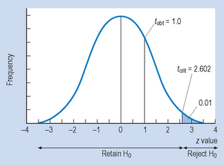
The previous two examples involved sample sizes of n > 30. However, as we saw in Chapter 17, if n < 30, the distribution of sample means is not a normal, but a t distribution. This point must be taken into account when we calculate the probability of H₀ being true. That is, for small samples, we use the t test to evaluate the significance of our data.

  Page 214 

Assume exactly the same information as in Example 1, except that sample size is n = 16.

1. Directional H_A: as in Example 1.

2. H₀: as in Example 1.

3. α = 0.01, one tail.

4. We can find from the t table (Appendix B) the value for t_crit. To look up t_crit we must have the following information:

(a) α, the level of significance (0.05 or 0.01)

(b) direction of H_A (directional or nondirectional)

(c) the degrees of freedom (df).

In this instance:

(a) α = 0.01

(b) H_A is directional, therefore we must look up a one-tail probability

(c) df = n − 1 = 16 − 1 = 15

Looking up the appropriate value for t; t_crit = 2.602. Calculating the t score (t_obt) representing the probability of the sample being drawn from the population under H₀, we use the formula:

5. As we stated earlier, the decision rule is identical to that of the z test:

Here, 1.0 < 2.602, such that t_obt falls into the area of retention (Fig. 18.6). Therefore, we must retain H₀ at a 0.01 level of significance. Clearly, when n = 16, the investigation did not show a significant weight increase for the males.

Figure 18.6 Hypothesis testing: directional.

Conclusion

The above examples demonstrate the following points about statistical decision making:

• We are more likely to reject H₀ if we use a one-tail test (directional H_A) than a two-tail test (non-directional H_A). In effect, we are using the prediction of which way the differences will go to increase the probability of rejecting H₀ and therefore accepting H_A. Examples 1 and 2 demonstrate this point; in Example 1 we rejected H₀ with a directional H_A, while we retained H₀ in Example 2, with exactly the same data.

• The larger the sample size, n, the more likely we are to reject H₀ for a given set of data. Comparing Examples 1 and 3 demonstrates this; although μ, σ, and were the same, where n was small we had to retain H₀. Also, when n is small, (n < 30), we must use the t test to analyse the significance of our sample mean being different.

• The more demanding the decision level (that is, if α is small), the less likely we are to reject H₀. To illustrate this point, repeat Example 2, but set α = 0.05. Here, z_crit = 1.96 so that z_obt is greater than z_crit. Therefore, we can reject H₀, and accept H_A at a 0.05 level of significance. That is, with exactly the same data, we have rejected or accepted H₀, depending on the level of significance, α.

Errors in inference

When we say our results are statistically significant, we are making the inference that the results for our sample are true for the population. It should be evident from the previous discussion that statistical decision making can result in incorrect decisions. There are two main types of inferential error: Type I and Type II.

A Type I error occurs when we mistakenly reject H₀; that is, when we claim that our experimental hypothesis was supported when it is, in fact, false. The probability of a Type I error occurring is less than or equal to α. For instance, in the previous Example 1 we set α = 0.01. The probability of making a Type I error is less than or equal to 0.01; the chances are equal to or less than 1/100 that our decision in rejecting H₀ was mistaken. Therefore, the smaller α, the less the chance of making a Type I error. We can set α as low as possible, but by convention it must be less than or equal to 0.05.

A Type II error occurs when we mistakenly retain H₀; that is, when we falsely conclude that the experimental hypothesis was not supported by our data. The probability of a Type II error occurring is denoted by β (beta). In Example 3 we retained H₀, perhaps falsely. If n was larger, we might well have rejected H₀, as in Example 1. Type I errors represent a ‘false alarm’ and Type II errors represent a ‘miss’. Table 18.2 illustrates this.

Table 18.2 Decision outcomes

Table 18.2 illustrates that, if we reject H₀, we are making either a correct decision or a Type I error. If we retain H₀, we are making either a correct decision or a Type II error. While we cannot, in principle, eliminate these from scientific decision making, we can take steps to minimize their occurrence.

We minimize the occurrence of Type I error by setting an acceptable level for α. In scientific research, editors of most scientific journals require that α should be set at 0.05 or less. This convention helps to reduce false alarms to a rate of less than 1/20. Replication of the findings by other independent investigators provides important evidence that the original decision to reject H₀ was correct.

How do we minimize the probability of Type II error?

2. Reduce the variability of measurements (s, either by increasing accuracy (Ch. 12) or by using samples that are not highly variable for the measurement producing the data).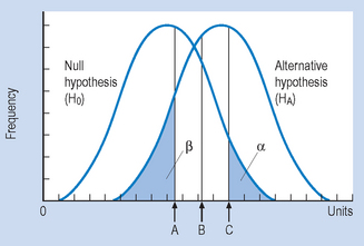

Figure 18.7 Change of decision level to increase β and decrease α. As the decision criterion is moved from A to B to C, the relative frequency of Type I and Type II errors alters.

Summary

The problem addressed in the previous two chapters was that, although our hypotheses are general statements concerning populations, the evidence for verifying or supporting our hypotheses is based on sample data. We solve this problem through the use of inferential statistics.

It was argued in this chapter that, once the sample data have been collected and summarized, the investigator must analyse the findings to demonstrate their statistical significance. Significant results for an investigation mean that differences or changes demonstrated were real, rather than just the outcome of random sampling error.

The general steps in using tests of significance were explained, and several illustrative examples using the z and t tests for single sample designs were presented. A critical value is set for the statistic (in this case z_crit, t_crit) as specified by α. If the magnitude of the obtained value of the statistic (z_obt, t_obt) exceeds the critical value, H₀ is rejected. In this case, the investigator concludes that the data supported the differences predicted by the alternative hypothesis (at the level of significance specified by α). However, if the obtained value of the statistic is calculated to be less than the critical value, then the investigator must conclude that the data did not support the hypothesis. It was noted that following these steps does not guarantee the absolute truth of decisions made about the rejection or acceptance of the alternative hypotheses, but rather specifies the probability of the decisions being correct.

Two types of erroneous decisions were specified, Type I and Type II errors. A Type I error involves falsely concluding that differences or changes found in a study were real, that is, concluding that the data supported a hypothesis which is, in fact, false. A Type II error involves falsely concluding that no differences or changes exist, that is, concluding that the data did not support a hypothesis which is, in fact, true. It was demonstrated that the probability of these errors depends on factors such as the size of n, the directionality of H_A and the variability of the data.

The procedures of hypothesis testing and error were related to the logic of clinical decision making. The probabilities (α and β) of making Type I and Type II errors are interrelated. In this way, both researchers and clinicians must take into account the implications of possible error when setting levels of significance for interpreting the data.

Self-assessment

Explain the meaning of the following terms:

Multiple choice

1. Hypothesis testing involves:

a deciding between two mutually exclusive hypotheses, H₀ and H_A

b deciding if the investigation was internally and externally valid

c deciding if the differences between groups was large or small

d none of the above.

2. An α level of 0.01 indicates that:

a the probability of falsely rejecting H₀ is limited to 0.05

b the probability of Type II error is 0.01

c the probability of a correct decision is 0.01

d none of the above.

3. If α is changed from 0.01 to 0.001:

a the probability of making a Type II error decreases

b the probability of a Type I error increases

c the error probabilities stay the same

d the probability of a Type I error decreases.

4. If we reject the null hypothesis, we might be making:

a a Type II error

b a Type I error

c a correct decision

d a or c

e b or c.

5. Statistical tests are used:

a only when the investigation involves a true experimental design

b to increase the internal validity of experiments

c to establish the probability of the outcome of an investigation being due to chance alone

d a and b.

6. The outcome of a statistical analysis is found to be p = 0.02. This means that:

a the alternative hypothesis was directional

b we can reject H₀ at α = 0.05

c we must conclude that H_A must be true

d a and c.

7. When the results of an experiment are nonsignificant, the proper conclusion is:

a the experiment fails to show a real effect for the independent variable

b chance alone is at work

c to accept H₀

d to accept H_A.

8. It is important to know the possible errors (Type I or Type II) we might make when rejecting or failing to reject H₀:

a to minimize these errors when designing the experiment

b to be aware of the fallacy of accepting H₀

c to maximize the probability of making a correct decision by proper design

d all of the above.

9. An α level of 0.05 indicates that:

a if H₀ is true, the probability of falsely rejecting it is limited to 0.05

b 95% of the time chance is operating

c the probability of a Type II error is 0.05

d the probability of a correct decision is 0.05.

10. A directional alternative hypothesis asserts that:

a the independent variable has no effect on the dependent variable

b a random effect is responsible for the differences between conditions

c the independent variable does not have an effect

d there are differences in the data in a given direction.

11. If α is changed from 0.05 to 0.01:

a the probability of a Type II error decreases

b the probability of a Type I error increases

c the error probabilities stay the same

d the probability of Type II error increases.

12. If the null hypothesis is retained, you may be making:

a a correct decision about the data

b a Type I error

c a Type II error

d a or c

e a or b.

  Page 218 

13. When the results are statistically significant, this means:

a the obtained probability is equal to or less than α

b the independent variable has had a large effect

c we can reject H₀

d all of the above

e a and c.

14. β refers to:

a the probability of making a Type I error

b the probability of (1 − α)

c the inverse of the probability of sampling error

d the probability of making a Type II error.

15. Setting α = 0.0001 would reduce the probability of Type I error. However, it would:

a increase Type II error probability

b increase the standard error of variance

c reduce external validity

d all of the above.

16. We retain H₀ if:

a | t_obt | ≤ | t_crit |

b | t_obt | > | t_crit |

c | t_obt | < | t_crit |

d none of the above.

17. If α is changed from 0.01 to 0.001:

a the probability of a Type II error decreases

b the probability of a Type I error increases

c the error probabilities stay the same

d none of the above.

A researcher believes that the average age of unemployed people has changed. To test this hypothesis, the ages of 150 randomly selected unemployed people are determined (A). The mean age is 23.5 years. A complete census taken a few years before showed a mean age of 22.4 years, with a standard deviation of 7.6 (B).

Questions 18–22 refer to these data.

18. The alternative hypothesis should be:

a _A = _B

b μ_A = μ_B

c μ_A # μ_B

d _A # _B

19. The z_crit where α = 0.01 is:

a + 2.58

b + 1.64

c + 2.33

d − 1.64

20. The obtained value of the appropriate statistic for testing H₀ is:

a 2.88

b 2.35

c 1.84

d 1.77

21. What do you decide, using α = 0.01?

a retain H₀

b reject H₀

c it is not possible to decide

d a and b.

22. Therefore, the researcher should conclude that:

a unemployed persons are getting older on average

b there is no evidence supporting the hypothesis that the average age of unemployed people has changed

c too many young people are unemployed

d b and c.

23. When the results are not statistically significant, this means that:

a the experimental hypothesis was not supported by the data at a given level of probability

b the null hypothesis was retained at a given level of probability

c the alternative hypothesis must have been directional

d the investigation was internally valid

e a and b.

24. If α = 0.05 and the probability of the statistic calculated from the data is p = 0.02, then:

a we should retain H₀

b we should reject H_A

c we should reject H₀ at α = 0.05

d we should restate H₀ so that the findings will become significant at the 0.05 level.