Introduction

In the previous chapter, we examined the logic of hypothesis testing and the use of z and t tests for testing hypotheses about single sample means. There are numerous statistical tests available which are used in a conceptually similar fashion to analyse the statistical significance of the data. That is, all statistical tests involve setting up the relevant hypotheses, H₀ and H_A, and then, on the basis of the appropriate inferential statistics, computing the probability of the sample statistics obtained occurring by chance alone. We are not going to attempt to examine all statistical tests in this introductory book. These are described in various statistics text books or in data analysis manuals. Rather, in this chapter we will examine the criteria used for selecting tests appropriate for the analysis of the data obtained in specific investigations. To illustrate the use of statistical tests we will examine the use of the chi-square test (χ²). This is a statistical test commonly employed to analyse nominally scaled data. Finally, we will briefly examine the uses of the Statistical Package for Social Sciences (SPSS) for data analysis in general.

The aims of this chapter are to:

The relationship between descriptive and inferential statistics

As we have seen in the previous chapters, statistics may be classified as descriptive or inferential. Descriptive statistics are concerned with issues such as ‘What is the average length of hospitalization of a group of patients?’ Inferential statistics are used to address issues such as whether the differences in average lengths of hospitalization of patients in two groups are statistically significantly different. Thus, descriptive statistics describe aspects of the data such as the frequencies of scores, the average or the range of values for samples, whereas when using inferential statistics, one attempts to infer whether differences between groups or relationships between variables represent persistent and reproducible trends in the populations.

In Section 5 we saw that the selection of appropriate descriptive statistics depends on the characteristics of the data being described. For example, in a variable such as incomes of patients, the best statistics to represent the typical income would be the mean and/or the median. If you had a millionaire in the group of patients, the mean would give a distorted impression of the central tendency. In this situation the median would be most appropriate. The mode is most commonly used when the data being described are categorical. For example, if in a questionnaire respondents were asked to indicate their sex and 65 said they were male and 35 female, then ‘male’ is the modal response. It is quite unusual to use the mode only with data that are not nominal. As a rule, the scale of measurement used to obtain the data and its distribution determine which descriptive statistics are selected.

In the same way, the appropriate inferential statistics are determined by the characteristics of the data being analysed. For example, where the mean is the appropriate descriptive statistic, the inferential statistics will determine if the differences between the means are statistically significant. In the case of ordinal data, the appropriate inferential statistics will make it possible to decide if either the medians or the rank orders are significantly different. With nominal data, the appropriate inferential statistic will decide if proportions of cases falling into specific categories are significantly different.

Thus, when the data have been adequately described, the appropriate inferential statistic will follow logically. However, when selecting an appropriate statistical test, the design of the investigation must also be taken into account.

Selection of the appropriate inferential test

Before addressing the issue of the selection of the appropriate inferential statistical test, it is useful to reiterate the reason why a statistical test should be employed.

In many studies, inferential statistical tests are not required. For example, if a health care needs-assessment survey is conducted in a particular community, using a full population, the investigator might not be overly concerned with generalizing the results to other communities, or with demonstrating that certain relationships between variables are reliable. It may be enough to be able to say, for example, that ‘35% of the respondents indicated that they were dissatisfied with the existing level of medical services’. In this instance, descriptive statistics are all that the investigator requires since the complete population was studied. If, however, the investigator wishes to argue that certain differences between groups or that certain correlations between variables for a sample are generalizable to the population, then inferential statistical tests are necessary.

The inferential statistic provides the investigator with a means of determining how reproducible the obtained results are, by enabling access to a probability. The probability associated with the value of an inferential statistic informs the investigator of the likelihood that the results obtained were due to chance factors, or if they are significant at a given level of probability.

Please note that we are not going to examine all of the numerous statistical tests available for decision making. Rather, the aim of this chapter is to examine the criteria used for selecting tests appropriate for the analysis of data obtained in investigations. To illustrate the use of statistical tests we will look at the χ² test, commonly employed for analysing nominal data. We examine the interpretation of findings which do not reach statistical significance and the relationship between statistical and clinical significance. In Chapter 20 we will consider some of the personal and social values implicit in making decisions concerning the actual adoption and use of treatments and diagnostic tests in clinical settings.

There is a variety of statistical tests, some of which are named in Table 19.1. The selection of the appropriate statistical test is determined by the following considerations:

Table 19.1 Selection of tests of significance

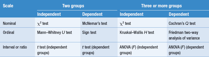
Table 19.1 offers a sample of statistical tests in order to illustrate how statistical tests are selected for analysing data. Several points are worth noting.

Let us look at some examples to illustrate how statistical tests are selected.

An investigator wishes to evaluate the effectiveness of a new treatment in contrast to a conventionally used treatment. Assume that the outcome (dependent variable) is measured on a five-point ordinal scale. Each subject is assigned to one of the two treatment groups. Which test would the investigator use to analyse the significance of sample data when:

By inspection of Table 19.1 the investigator would select the Mann–Whitney U test to analyse the significance of the data.

If we change the above example by stating that the dependent variable was measured on an interval scale, the appropriate test would now be a t test (for independent groups). Let us say that three groups were used (by the inclusion of a placebo group) by the investigator. Now, if the outcome measurement remained ordinal, the appropriate test for analysing the data is the Kruskal–Wallis H test. If, however, the outcome measures were interval, it follows from Table 19.1 that the appropriate test for analysing the results would be ANOVA (analysis of variance).

Finally, say that in the original example each of the subjects was treated with both the new and old treatments. Now, the data would have been obtained from the repeated measurement of the same subjects, and the appropriate statistical test would be the Sign test (ordinal, two groups, dependent).

Table 19.1 does not include all the available statistical tests and their uses. In fact, mathematical statisticians can generate inferential tests appropriate for a whole variety of designs. The basic idea is to use probability theory to generate appropriate sampling distributions in terms of which the probability of H₀ being true can be calculated, and the statistical significance of the findings evaluated.

Rather than examining all the tests and their underlying assumptions, we will look at the use of the χ² test in some detail. As well as being a very useful test for analysing nominal data, it (along with the z and t) illustrates how statistical tests are carried out to test hypotheses.

The χ² test

As shown in Table 19.1, χ² (chi-square) is appropriate for statistical analysis when:

The χ² test is appropriate for deciding if proportions of cases falling into categories are different at a given level of significance.

The statistic, χ², is given by the formula:

where f_o = observed frequency for a given category and f_e = expected frequency for a given category, assuming H₀ was true.

The sampling distribution for χ² is a family of curves, which, like t, vary with degrees of freedom. The use of this inferential statistic is best illustrated by an example.

Suppose that an investigator is interested in finding out whether there is a difference in the relative frequency of different kinds of treatments currently offered to extremely depressed patients. A random sample of 150 patients is selected from a population of patients in Australia, and the type of treatment offered to them is determined from their medical records, as shown in Table 19.2.

Table 19.2 Treatments offered

The entries in each cell represent the frequency with which patients were given the various treatments. Thus, 45 patients were offered psychotherapy, 40 drugs and 65 electroconvulsive therapy. The χ² is the appropriate test for analysing these data. Let us follow the steps involved in hypothesis testing, as outlined in Chapter 18.

Here, χ²_crit is the critical value of the statistic χ², which cuts off a proportion of the sampling distribution equal to α. The value of χ²_crit is obtained from the tables in Appendix C. To look up this statistic, we need to know:

Note that with χ² the degrees of freedom with one variable is k − 1, where k stands for the number of categories or groups. In this instance, we have k = 3 (three treatments) so that df = 3 − 1 = 2. Now we can look up the tables in Appendix C. In this case, α = 0.05 and df = 2, therefore χ²_crit = 5.99.

Here, since χ²_obt > χ²_crit we can reject H₀ at a 0.05 level of significance. The investigator is in a position to accept H_A (that the three treatments are offered at different frequencies to depressed patients). Clearly, electroconvulsive therapy is given most frequently for the condition (in this hypothetical example).

χ² and contingency tables

In the previous example of χ² we had clear expectations of the expected frequencies (f_e) and were dealing with only one variable. The χ² test is also relevant for analysing nominal data where f_e is not known, and where we are interested in the effects of more than one variable. Thus, χ² is a statistical test appropriate for deciding whether two variables are significantly related.

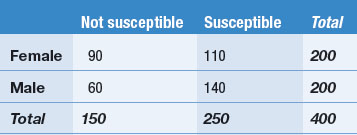
For example, an investigator compares the effectiveness of drug therapy with coronary artery surgery in males 55–60 years old, suffering from coronary heart disease. A sample of 40 patients consenting to the investigation is selected from this population, and randomly divided into the two treatment groups (drugs only or coronary artery surgery). The treatment outcome is measured in terms of survival over 5 years. The outcome of this hypothetical study is shown in Table 19.4.

Table 19.4 Contingency table showing obtained frequencies for a hypothetical study comparing survival after treatments

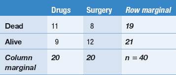
Table 19.4 is called a contingency table. A contingency table is a two-way table showing the relationship between two or more variables. Note that the levels of the variables have been classified into mutually exclusive categories (‘drugs or surgery’ for the independent variable, and ‘dead or alive’ for the dependent variable, in this instance). The cells in the contingency table show the frequency of cases falling into each joint category (for example, 11 people who had ‘drugs only’ died during the 5 years). The row and column marginal scores are the sums of the frequencies. The row and column marginals necessarily add up to n, the sample size (n = 40 for this example).

Table 19.4 is called a two-by-two (2 × 2) contingency table. Depending on the number of categories (or levels) in each of the two variables, we might have 3 × 2 tables, 3 × 3 tables, etc. Let us now turn to analysing the data.

5. Making decisions concerning H₀: the degrees of freedom for a contingency table are calculated by the following formula:

Table 19.6 Sample calculation of chi-squared

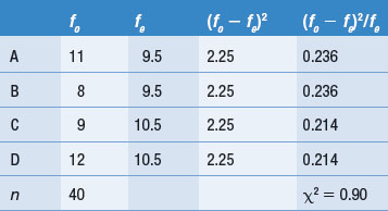
where r = the number of rows and c = the number of columnsa. In this instance, given a 2 × 2 contingency table:

Now we can look up χ²_crit, for α = 0.05 and df = 1. From Appendix C, χ²_crit = 3.84. Therefore, since χ²_obt < χ²_crit we must retain H₀: there is no statistically significant difference in the frequencies of survival over 5 years following the two kinds of treatments. Our data show that either there is no difference in the outcomes of the two treatments or we made a Type II error.

The χ² test can be used to analyse the statistical significance of nominal data arising from experimental or non-experimental investigations. This non-parametric test can be used provided that two simple assumptions are met:

If either of these assumptions is violated, the use of χ² is inappropriate for statistical decision making. Assumption 2 is particularly important when the degrees of freedom is one (df = 1) for a contingency table.

Statistical packages

We have been looking at a few simple examples of establishing the statistical significance of the results. These calculations were presented only for teaching purposes. Some older applied statistics text books are crammed with complicated formulae for calculating dozens of different inferential statistics. Researchers now use statistical packages which have made statistical analysis simpler and more accessible to all researchers. The following steps are followed when using statistical packages:

Select a statistical package

There are many packages on the market, including Statistical Package for Social Sciences (‘SPSS’), ‘STATISTICA’, ‘Statsview’ or various spreadsheets with useful statistical functions. Each program has its strengths and weaknesses and some researchers have formed strong attachment to specific programs. If you are a beginner, you should be guided by your thesis supervisor or your workplace mentor about the availability of packages.

Training

It is useful to learn how to use a package before you begin data analysis. Depending on your aptitude and experience, training sessions take 1 or 2 days. With more complex scientific packages such as ‘STATISTICA’ it might require long-term usage before one feels like an expert user.

Encode the raw data

Using all packages we begin by encoding the data. You have to be clear about issues such as which are your independent or dependent variables or the scaling of the data (continuous/discontinuous). That is, designs and measurement procedures used in your research project influence the encoding process (e.g. Schwartz & Polgar 2003, Ch. 1).

Identifying the statistical analysis required

Some degree of statistical knowledge is required beyond that covered in this book to enable you confidently to select and interpret the appropriate statistical analyses. Keep in mind that our book is introductory; it is expected that you will complete a more advanced statistics subject. For more complex analyses it might be useful to seek expert help.

Printout

You will select the appropriate statistical analysis from the ‘menu’ and print out the results of the analysis.

Interpretation

Finally you will need to interpret the ‘printout’ in relation to your research questions and/or hypotheses.

Let us look at a simple example. Say we are interested in the benefits of exercise for improving mobility in nursing home residents. A sample of 24 (n = 24) residents with reduced mobility are selected and give informed consent to participate. The participants are randomly assigned to either of two groups: ‘E’, which involves them undertaking an exercise programme suitable for improving mobility in elderly patients, and ‘C’, which involves undertaking alternative activities of equal duration. The outcome or dependent variable is measured as the distance in metres safely walked by the residents unassisted at the completion of the exercise and control programmes. The research hypothesis here is: exercise improves mobility in nursing home residents. We will look at a set of created data to illustrate hypothesis testing using a statistical package (SPSS).

  Page 226 

Let us follow the steps for analysing the data:

1. Assume that the SPSS package is readily available in your workplace and you are informed by your computing expert or supervisor.

2. You have had some training. Even if no formal training is available, self-help books such as SPSS: Analysis Without Anguish. Version 11.0 for Windows (Coates & Steed 2003) are very useful.

3. After accessing the spreadsheet for the program, we encode the data in the two columns representing ‘E’ and ‘C’. We inform the program that the data are ‘continuous’ (ratio-scale data).

4. We refer to Table 19.1 to identify the required statistical analysis. Here we have:

• two groups

• independent groups

• ratio-scale data.

Therefore, we select the independent t test for analysing the data from the ‘menu’ of inferential tests available.

5. Printouts: Tables 19.7 and 19.8 for SPSS are based on printouts presented in Coates & Steed (2003, p. 73). We changed the original example which contains additional information: the interested reader might wish to examine it further in Coakes & Steed (2003).

Table 19.7 Printout for descriptive statistics

Table 19.8 t test for equality of means

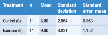
Table 19.7 shows key descriptive statistics:

• n refers to the sample size for each group

• mean () for each group

• standard deviation (s) for each group

• standard error mean (s_–x) for each group. You will recall from Chapter 17 . Here, for the control group ‘C’ the standard error mean = , as shown in the printout.

The group mean for the exercise group does in fact indicate a better overall performance. However, we are justified in concluding that exercise in general produces improved mobility in nursing home residents. To answer this question we must look at the results of the t test, as shown in Table 19.8.

The following information was presented:

• The t obtained was − 0.695, the minus sign simply reflecting that the mean for the exercise group was less than the mean for the control group. A t value of 0.695 is quite ‘small’ in relation to the critical values for t shown in Appendix B.

• ‘df’ refers to degrees of freedom. For the control group’s t test, df = n₁ + n₂ − 2 (Schwartz & Polgar 2003). Here, df = 11 + 11 − 2 = 20, as shown in Table 19.8.

• ‘Sig. (2-tailed)’ refers to the probability of a difference between the means being obtained by chance, i.e. p (H₀ is true) (see Ch. 18). The decision rule is that we reject H₀ if p < 0.05. Here the calculated probability is 0.495 and therefore we retain H₀. We conclude that the results were not statistically significant.

• The ‘mean difference’ refers to the difference between the two sample means; that is, 8 − 9 = − 1, as shown in Table 19.8.

• ‘Standard error difference’ refers to the standard error of the distribution of sample means. We will not discuss this statistic in detail. However, as shown in Chapter 17, the standard error enables us to calculate a 95% confidence interval; in this case for –X_C − –X_E.

  Page 227 

• The lower and upper limits show that the true (i.e. population) difference (μ_C − μ_E) probably (p = 0.95) falls between − 4.003 and 2.003. This is a wide range for a confidence interval and therefore indicates that residents who exercise might be able to walk either four extra metres or, for that matter, two metres less than those who don’t exercise. Of course, any other difference between the two limits is possible. Clearly, such results are far too variable to attribute any clinical benefits to the exercise programme.

Summary

There are a variety of statistical tests available for analysing the significance of the obtained data. The statistical test appropriate for analysing a given set of data is selected on the basis of:

Generally, parametric and non-parametric statistical tests were distinguished on the grounds of the scaling of the data and the assumptions underlying the sampling distributions.

None of the individual statistical tests was discussed in detail, except the χ² test, which was presented as an example. Together with the discussion on the z and t tests in Chapter 18, the χ² test illustrates the principle that theoretical sampling distributions can be generated, and the probability of obtaining specific outcomes can be calculated. If the obtained value of the inferential statistic is greater than or equal to the critical value, the null hypothesis can be rejected at the level of significance specified by the Type I error rate (α). This is the case regardless of which particular statistical test is being used.

The retention of H₀ might reflect a correct decision, or a Type II error. Sample size is a factor which contributes to Type II error rate, as shown in both Chapters 18 and 20.

Self-assessment

Explain the meaning of the following terms:

Multiple choice

1. In a study, three independent samples are compared and the dependent variable is measured on a ratio scale. A statistical test appropriate for analysing these findings is:

a χ²

b Mann–Whitney U

c t

d ANOVA (analysis of variance).

2. In a study, two independent samples are compared and the dependent variable is measured on an ordinal scale. A statistical test appropriate for analysing these findings is:

a χ²

b Mann–Whitney U

c t

d Wilcoxon.

3. Which of the following is a ‘non-parametric’ test?

a ANOVA (analysis of variance)

b t

c z

d Kruskal–Wallis H.

4. Which of the following is a ‘parametric’ test?

a Median test

b McNemar’s test

c z

d Cochran’s Q.

5. Which of the following tests is appropriate for analysing data where three or more groups were used?

a z

b t

c χ²

d Sign test.

6. The larger the discrepancy between f_o and f_e for each cell in a contingency table:

a the more likely it is that the results will not be significant

b the more likely it is that H₀ will be rejected

c the more likely it is that the population proportions are the same

d the more likely it is that the population proportions are different

e a and c

f b and d.

7. For any given level of significance, χ²_crit:

a increases with increases in sample size

b decreases with increases in degrees of freedom

c increases with increases in degrees of freedom

d decreases with increases in sample size.

8. A contingency table:

a always involves two degrees of freedom

b always involves two dependent frequencies

c always involves two variables

d all of the above

e a and b.

9. Entries into the cells of a contingency table should be:

a frequencies

b means

c percentages

d degrees of freedom.

10. The degrees of freedom for a contingency table:

a equal n − 1

b equal rc − 1

c cannot be determined if r = c

d equal (r − 1) (c − 1).

11. χ² should not be used with a 2 × 2 contingency table if:

a df > 1

b f_e is below 5 in any cell

c f_o is below 5 in any cell

d f_e = f_o

e b and c.

An investigator is interested in determining whether there is a relationship between gender and susceptibility to a substance known to trigger an allergic response. ‘Susceptibility’ is measured as yes or no.

Questions 12–15 refer to this example. The raw data are presented in the contingency table below.

  Page 229 

12. The value of χ²_obt is:

a 2.50

b 8.09

c 9.60

d 11.05

13. The value of df is:

a 2

b 1

c 3

d need more information.

14. Using α = 0.05, χ²_crit is:

a 3.841

b 5.412

c 2.706

d − 3.841

15. Using α = 0.05, what is your conclusion?

a Accept H₀: there is no relationship between gender and susceptibility.

b Reject H₀: there is a significant relationship between gender and susceptibility.

c Fail to reject H₀: the study does not show a significant relationship between gender and susceptibility.

d Fail to reject H₀: this study shows a significant relationship between gender and susceptibility.

16. In selecting an appropriate statistical test:

a z should be used as it is most powerful

b t should be used as it takes the sample size into account

c the choice depends on the design of the study

d χ² should be avoided.

17. The χ² test requires that:

a data be measured on a nominal scale

b data conform to a normal distribution

c expected frequencies are equal in all cells

d all of the above occur.

The following information should be used in answering questions 18–25. Aerobics classes are conducted by the student union of a tertiary institution; although there are equal numbers of male and female students enrolled at the institution, it is observed that far more female than male students attend. A test is performed to see whether the proportion of the two sexes at the class is representative of the proportion of the two sexes enrolled at the institution as a whole. Of the 50 students who attend the classes, 10 are male. A χ₂is conducted on these data.

18. What type of χ² will be conducted?

a one-way

b two-way

c contingency analysis

d parametric.

19. How many cells will there be in the χ² table?

a 1

b 2

c 3

d 4

20. What is the expected frequency of male students at the aerobic classes?

a 10

b 40

c 25

d 8

21. What is the obtained value of χ²?

a 4.5

b 2.5

c 18.0

d 9.0

22. What are the degrees of freedom?

a 1

b 2

c 49

d 48

23. If α is set at 0.01, what is the critical value of χ²?

a 0.0201

b 4.605

c 9.210

d 6.635

24. What statistical decision should be made on the basis of these data?

a Reject null hypothesis.

b Retain null hypothesis.

c Increase α.

d Increase size of sample.

  Page 230 

25. What conclusion can be drawn on the basis of these data?

a Overall, the tendency for more females than males to attend the classes is not statistically significant.

b There is a statistically significant tendency for more females than males to attend the classes (α = 0.01).

c The aerobics classes should have their format changed to attract more male students.

d There is a statistically significant trend (α = 0.01) for differential attendance by the two sexes, but it is impossible to state the direction of this trend.

The following information should be used in answering questions 26–31. In a test of the effectiveness of phenothiazine in treating schizophrenia, 60 patients are randomly assigned to receive either the drug or a placebo; after 2 weeks of daily treatment each patient is assessed by the chief psychiatrist as ‘improved’ or ‘not improved’. A 2 × 2 table is constructed to indicate improved number of patients falling into each category:

Assessment	Treatment
	Phenothiazine	Placebo
Improved	20	10
Not improved	10	20

26. The degrees of freedom in this table are:

a 1

b 2

c 3

d 4

27. The obtained χ² is:

a 1.33

b 13.5

c 8.71

d 6.67

28. With α set at 0.05, the critical value of χ² is:

a 3.841

b 5.991

c 6.635

d 0.013

29. The correct statistical decision in this case is to:

a reject H₀

b retain H₀

c decrease α

d increase α.

30. The appropriate conclusion to be drawn from these data is:

a Patients receiving the active drug are not significantly more likely to get an ‘improved’ rating than those receiving the placebo.

b Those receiving the active drug are significantly more likely to be rated as ‘improved’ (α = 0.05).

c The drug cures schizophrenia.

d The improvements cannot be due to the drug, as some people received the drug and did not improve.

31. Following the publication of this study, it is revealed that the psychiatrist who did the ratings of improvement was also the person who had assigned the patients to phenothiazine or placebo groups. What type of problem could have invalidated these findings?

a Rosenthal effects.

b Placebo effects.

c Instrumentation effects.

d All of the above.