Chapter 14 The AC transformer
Chapter contents
14.1 Aim
The aim of this chapter is to discuss the main concepts that govern the operation of the step-up or the step-down alternating current (AC) transformer. In addition to this, two forms of specialist transformers are discussed, namely the autotransformer and the constant-voltage transformer. Finally, there is an overview of the factors that affect transformer rating and how these factors relate to radiographic exposures.
14.2 Introduction
An AC transformer has an electrical input and an electrical output. For the transformer to function, the input is an AC supply. The electrical output potential difference may be either greater or smaller than the electrical input voltage. If the output voltage is greater than the input voltage, then the transformer is a step-up transformer; if it is less, then the transformer is a step-down transformer. A transformer is thus a device that changes ACs or voltages from one level to another.
The transformer has a wide range of applications in radiography. The mains voltage is too low to be applied directly across the X-ray tube and so it is increased using a step-up transformer (the high-tension transformer). On the other hand, the mains voltage is too high to be connected directly across the filament and so it is reduced in the filament transformer – an example of a step-down transformer. Two other types of transformer are encountered in radiography and so will be discussed in this chapter. These are the autotransformer and the saturated core or constant-voltage transformer.
14.3 The ideal transformer
Let us start by defining this device:
An ideal transformer is one whose output electrical power is equal to its input electrical power – there is no power ‘lost’ in the transformer itself.
There is, of course, no such thing as the ideal (or perfect) transformer, although real transformers with efficiencies of 98% or more are not uncommon. Although not a practical reality, the concept of the ideal transformer is a useful one in that it simplifies the mathematics which can be used to describe the behaviour of transformers.
Consider such an ideal transformer, shown in Figure 14.1, where two isolated sets of windings share a common core – there are a number of other configurations of core and windings but the one shown in Figure 14.1 is the simplest. The input or primary side of the transformer consists of np turns around the core and has an alternating voltage VP across it. The output or secondary side of the transformer consists of ns turns and has a voltage Vs induced in it. This is a case of mutual induction, as discussed in Section 10.7. The sequence of events is as follows:
• The alternating voltage in the primary winding VP causes an AC to flow through the winding.
• This AC, Ip, produces a changing magnetic flux density (B) in the soft iron core.
• The changing magnetic flux density is linked to the secondary winding so that an electromotive force (EMF), Vs, is induced in it according to Faraday’s and Lenz’s laws of electromagnetic induction (see Sects 10.4 and 10.5).
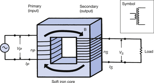
Figure 14.1 An ‘ideal’ transformer showing the core and the primary and secondary windings. In practice, the core is laminated, as shown in Figure 14.2. As there are more turns on the secondary winding than on the primary winding, this is a step-up transformer. The symbol for a step-up transformer is also shown. See text for details.
As already mentioned in the introduction to this chapter, an AC supply is essential for the operation of the transformer since no EMF will be generated in the secondary if the magnetic flux is constant (Faraday’s first law).
The purpose of the soft iron core is to contain all the magnetic flux within it so that the magnetic flux linkage between the primary and the secondary is as near perfect as possible. The core is able to do this because of its strong induced magnetism, resulting from its high magnetic permeability (see Table 14.1).
Table 14.1 A summary of the losses associated with a particular transformer
| TRANSFORMER LOSS | COMMENTS |
|---|---|
| Copper losses | Caused by the resistance of the copper windings. Also known as I2R losses |
| Iron losses | Losses produced in the transformer core |
| Imperfect magnetic flux linkage | Very small loss flux |
| Eddy currents | Caused by electromagnetic induction within the core of the transformer – reduced by core lamination |
| Hysteresis | Caused by the work required to move the magnetic domains – reduced by the appropriate choice of core material (e.g. stalloy) |
| Regulation (a consequence of all the above losses) | Output voltage decreases with increased current load because of the increased losses due to the resistance of the windings |
The mathematics of the ideal transformer are relatively simple if we first consider the effect of the magnetic flux on a single turn of wire around the core. Since we are assuming that the transformer is ideal, there is no magnetic flux loss and the EMF induced is independent of the position of the wire. Thus, the same voltage will be induced in each turn of the primary and in each turn of the secondary. If we call this voltage v, then we can say that the total primary voltage is the voltage in each turn multiplied by the number of turns. Thus:


Thus, we can combine the two equations above to get:

By cross-multiplying this equation, we get the formula:

Note: This equation is true for either peak or root mean square (RMS) values of the voltage, provided Vs and Vp are both expressed in the same units.
The ratio Vs/Vp is known as the voltage gain of the transformer. This is greater than unity for a step-up transformer and less than unity for a step-down transformer.
The ratio ns/npis known as the turns ratio of the transformer. Again, if this is greater than unity, we have a step-up transformer and if it is less than unity, we have a step-down transformer.
If we have a transformer with a turns ratio of 200:1, we know that there are 200 times as many turns on the secondary as on the primary and that the voltage across the secondary is 200 times that of the primary.
The current flowing in the secondary of the transformer may be calculated from the power in the primary winding and secondary winding (for simplicity, in the following discussion, RMS values are assumed). In the ideal transformer, the power in the primary and the power in the secondary are equal. Thus:

From Equation 14.1 we know:

Thus, for an ideal transformer, we can say:

14.4 Faraday’s laws and lenz’s law applied to transformers
We have already considered Faraday’s laws of electromagnetic induction (Sect. 10.4) and Lenz’s law (Sect. 10.5) and we can now look at how these are applied to transformers.
As discussed in the previous section, there is a changing magnetic flux produced by the alternating supply connected to the primary and, since this is linked to both the primary and secondary windings, by Faraday’s laws, an EMF is produced in each of the windings. Assuming we have an ideal transformer, the magnitude of the EMF in each turn of the primary winding is equal to the magnitude of the EMF in each turn of the secondary.
Lenz’s law may be used to determine the direction of the induced current in the secondary. As it acts to oppose the changing magnetic flux, it will be in the opposite direction to (180° out of phase with) the current in the primary. The eddy currents induced in the core (these will be discussed later in this chapter, as they are part of the transformer ‘losses’) will also be in the opposite direction to the primary current.
Some find it surprising that it is the current drawn from the secondary of a transformer that determines the primary current, especially as the secondary voltage for a given transformer is determined by the primary voltage. The explanation of this fact is as follows.
Consider a situation when the secondary winding is open circuit (it is not connected to anything), so no current can flow through it, although an EMF is induced across it. If we assume that we have an ideal transformer, then the same EMF will be induced by this magnetic flux in the primary winding and, by Lenz’s Law, this will be in the opposite direction to the forward-EMF. Thus, no current flows in the primary winding when the secondary current is zero.
If the secondary is now connected across an external circuit so that some current flows through it, this current, by Lenz’s law, will oppose the magnetic flux in the core. The core flux is reduced and so the back-EMF in the primary is reduced. The forward-EMF in the primary is now greater than the back-EMF and so a current flows. Thus, a current in the secondary has caused a current to flow in the primary, the relative magnitudes of each being given by Equation 14.2.
14.5 Transformers in practice
It is not possible to construct an ideal transformer, as there are always power ‘losses’ within the transformer itself. This means that the power in the secondary is always less than the power in the primary by an amount equal to the transformer losses. The efficiency of a transformer may be defined as follows:
Note: It is often convenient to express the transformer efficiency as a percentage. For example, if a transformer is 95% efficient and 100 watts of power is supplied to the primary of that transformer, then 95 watts is produced in the secondary. In this case, 5% of the power is ‘lost’ because of power loss in the windings and core, i.e. this 5% is not available as useful electrical power.
Equation 14.1 gives a reasonable estimate of the voltage change in practical transformers but Equation 14.2 no longer applies because of the power losses in practical transformers. This may be illustrated by the following example.
A transformer has a turns ratio of 100:1 and an efficiency of 95%. If a current of 5 ARMS flows in the primary when a voltage of 10 VRMS is applied across it, what is the output RMS voltage and output RMS current?
From Equation 14.1 we get:

We also know that efficiency is the ratio of the output power to the input power. Thus:
Note that an ideal transformer would have produced the same secondary voltage but the secondary current would be 50 mARMS.
14.6 Transformer losses
A detailed analysis of the sources of transformer losses is considered in this section. These are summarized in Table 14.1 (See page. 84) and discussed below.
14.6.1 Copper losses
The term copper refers to the copper wire of the windings of the transformer, which has a small but finite resistance. If we consider a current IRMS flowing through a resistance R, then there is a power of (IRMS)2R watts produced within the resistor. (The copper loss is often referred to as the I2R loss of the transformer.) The copper loss produces a small heating effect within the coils of the transformer.
We wish to keep the copper loss as low as possible and, as it is related to I2R, it makes sense to keep R low when I is large. As we saw in Chapter 7, the resistance of a conductor is inversely proportional to its cross-sectional area. For this reason, the winding of the transformer, which carries the larger current, is made of the thicker wire. In the step-up transformer, this is the primary winding while in the step-down transformer it is the secondary winding.
14.6.2 Iron losses
The term iron losses refer to the losses that occur in the soft iron core of the transformer. These take three forms, as outlined below.
14.6.2.1 Magnetic flux losses
If the iron core is magnetically saturated, then all of the magnetic flux will not be contained within the core. This means that magnetic flux will be produced by the primary, which is not linked with the secondary. The EMF induced in the secondary and the output electrical power will be lower than if the flux linkage were perfect. By the appropriate design of the transformer core, in practice this loss is made very small indeed and so can be neglected for most practical purposes.
14.6.2.2 Eddy currents
From Faraday’s and Lenz’s laws, we know that when a changing magnetic flux is linked with a continuous conductor, an EMF and current are induced in the conductor. Also, the direction of the induced current opposes the effect of the changing magnetic flux linkage. The iron core of the transformer is a continuous electrical conductor and so the varying flux passing through the core will induce electric currents within the core itself in such a direction as to oppose the changing magnetic flux within the core. This principle is shown in Figure 14.2A where the direction of the eddy currents in the core is in the opposite direction to the current in the winding. The effect of these currents is two-fold:
1. The flow of electrical current through the core causes heating of the core due to the electrical resistance of the core.
2. The magnetic flux associated with the eddy currents is in the opposite direction to the flux from the winding and so there is a reduction in the flux interlinking with the secondary – flux which interlinks with the secondary is the flux produced at the primary minus the eddy current flux. This constitutes a power loss within the transformer core.
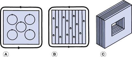
Figure 14.2 (A) Flow of eddy currents in an unlaminated transformer core. If the core is laminated, as shown in (B) and (C), then the eddy current flow is restricted and so the eddy current losses are limited.
Eddy currents may be reduced but not entirely eliminated by lamination of the core, as shown in Figure 14.2B and C. The laminated sheets of soft iron are bolted together to produce the required cross-sectional area. Each lamination is insulated from its neighbours by the application of a thin layer of insulation (e.g. polyester varnish) to its surface. This means that the eddy currents produced in the core are now confined to the small cross-sectional area of each lamination. As resistance is inversely proportional to cross-sectional area, lamination produces an increase in resistance and a consequent reduction in the size of the eddy current. There is, however, some eddy current present and this causes heating of the transformer core. Because of this, the transformer core requires to be cooled either by air or by immersing the transformer in oil, the latter acting as both a coolant and an insulator.
14.6.2.3 Hysteresis losses
Hysteresis is the lagging-behind of the induced magnetism in a ferromagnetic material when the applied magnetic field changes. Consider the changes which will occur in a transformer core during 1½ cycles of AC. The magnetizing force H changes with the current (see Fig. 14.3A). This produces changes in the magnetic intensity I as shown in Figure 14.3B. This graph is referred to as a hysteresis loop and the shape and size of this loop are important in the function of the transformer. The shape of this loop is explained as follows.
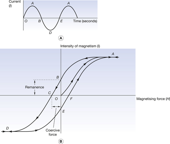
Figure 14.3 (A) Typical alternating current supply for a transformer winding; (B) hysteresis loop for a ferromagnetic sample. For an explanation of the connection between the two, see the text.
Consider a situation where the core is initially unmagnetized. As the magnetic domains are in randomized directions, there is no magnetic intensity within the core. This represents the origin O on both of the graphs. The current increases until it reaches its peak value at point A. The magnetizing force increases with the current and so initially does the magnetic intensity. This, however, flattens as magnetic saturation of the sample occurs so that the line is horizontal at point A on the hysteresis graph. The current now follows the curve AB and, as the magnetizing force decreases, so the magnetic intensity reduces along the curve AB on the hysteresis graph. Note that at point B, the magnetizing force is zero but there is still some magnetic intensity left in the ferromagnetic core sample. This magnetic intensity is known as the remanence in the core. To get rid of this remanence – so completely demagnetizing the core – a coercive force, represented by OC, must be used. Because the current has been reversed, the magnetizing force is also reversed and this continues until magnetic saturation is again produced at D. This occurs at the negative peak value of the current. As the current is reduced, the magnetizing force is again reduced and it is zero when the current is at point E on the graph of current. At this point on the hysteresis graph, there is again a remanence represented by OE (equal and opposite to OB) and this must be destroyed by the coercive force OF. The magnetizing force now continues to its positive peak, A, and the magnetic intensity follows the curve FA. The hysteresis loop is now complete.
The area of the hysteresis loop is important as it represents the work done in taking the sample through a complete hysteresis cycle. In considering the transformer core, the smaller the amount of work done, the smaller the iron loss from hysteresis. This should become clearer if we consider the hysteresis loops for soft iron and for steel.
Figure 14.4 shows the differences in the hysteresis loops for soft iron and steel. These differences may be summarized as follows:
• The saturation of soft iron occurs at much lower values of magnetizing force than the saturationof steel.
• The value of the coercive force is much greater for steel than for soft iron.
• The area of the hysteresis loop is much greater for steel than for soft iron.

Soft iron is therefore suitable for situations where a strong induced magnetism is required with the minimum expenditure of energy, and where the induced magnetism may be switched off at will. Note that, although the remanence is greater for soft iron than for steel, the coercive force is so small that a slight agitation of the sample will cause it to demagnetize. Suitable applications for soft iron are transformer cores (used as an alloy – stalloy).
Steel is a more suitable material for permanent magnets since it has a higher coercive force than soft iron and is thus more difficult to demagnetize. The high coercive force and the large area of the hysteresis loop make it unsuitable for use in the transformer core.
Subsidiary hysteresis loops. It is not necessary to take a ferromagnetic sample around a complete hysteresis loop, i.e. from magnetic saturation one way to magnetic saturation the other. In such cases, subsidiary hysteresis loops result, as shown in Figure 14.5. This is the type of hysteresis loop produced in most transformers – the exception being the saturated core transformer, which produces a complete hysteresis loop. The material with the hysteresis loop with the smallest area is still the most appropriate core material for a transformer.
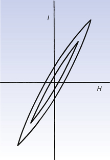
Figure 14.5 Subsidiary hysteresis loops where the ferromagnetic sample is not taken to full magnetic saturation.
The material usually selected for transformer cores is stalloy or permalloy as their small hysteresis loops limit the hysteresis ‘loss’. The power loss due to hysteresis in the core increases the kinetic energy of the atoms of the core and so manifests itself in the form of heat.
14.6.3 Regulation
Regulation in a transformer is a consequence of the resistance of the windings. If the electrical load drawn from the secondary is increased– a higher current is made to flow in the secondary – it is found that the potential difference across the secondary is decreased. This effect is termed transformer regulation.
Regulation occurs in any source of electricity which contains an internal resistance. In the case of the transformer, the internal resistance is the resistance of the secondary winding. Figure 14.6 shows a graph of the voltage output from a given transformer for differing secondary currents. The output current is zero when the secondary is open circuit. This corresponds to the open-circuit voltage (V0 in Fig. 14.6). In this condition, the transformer has zero regulation, it behaves as an ideal transformer and so Equation 14.1 may be used to calculate the secondary voltage. When the secondary of the transformer is connected to a load, current will flow in the secondary winding and the output voltage falls linearly with the secondary current. The transformer regulation therefore varies with the transformer load and so the output current is usually quoted with the regulation, e.g. ‘a transformer has a regulation of 2% when the secondary current is 400 mA’. The regulation is often expressed as a percentage and may be defined as follows:
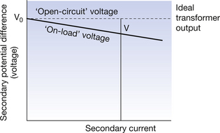
Figure 14.6 The greater the current drawn from the secondary winding of the transformer, the smaller becomes the potential difference across it. This effect is caused by the resistance of the transformer windings and is known as transformer regulation.
In Figure 14.6:
Most transformers used in radiography have a low percentage regulation and so the on-load voltage is close to the open-circuit voltage. In the case of the high-tension transformer, however, there must be a correction for this regulation, otherwise there would be a fall in the kVp if the tube mA was increased. Such corrections are made by compensating circuits, which are beyond the scope of this text.
The primary winding of a step-up transformer has such a low resistance that its effect on regulation may be ignored. If an EMF of V0 is induced in the secondary and the secondary resistance is r, then a current I will produce a voltage drop of Ir (Ohm’s law: V=IR) across the internal resistance r. This means that the potential difference which is available to the external circuit has been reduced by an amount Ir. Thus:

This formula should explain why the regulation is linear with the current, as shown in Figure 14.6. It should also be noted that when the secondary is ‘open-circuit’ then the secondary current is zero and so the voltage drop because of the internal resistance is zero. In such a situation, V=V0.
14.7 The autotransformer
The autotransformer permitted the operator to manually select a range of output voltages values whose values not very different from those of the input voltage (usually differing by a factor of between 0.5 and 2.0). Its principle function was to compensate for these slight variations, providing stable operating conditions for the other circuits of the X-ray generator. For this reason it is more commonly known as ‘the mains compensator’. The autotransformer consisted several turns forming single winding connected to the incoming mains supply. The changing magnetic flux of the AC supply produces an EMF in the winding which is evenly distributed over every turn of the winding. In accordance with Lenz’s Law (see Chapter 10) a back EMF is also produced the position of S2 in Figure 14.7 permits the operator to select a limited number of turns on the winding tapping the back EMF which has been produced in accordance with Lenz’s Law, thus producing a secondary voltage Vs and secondary current Is.
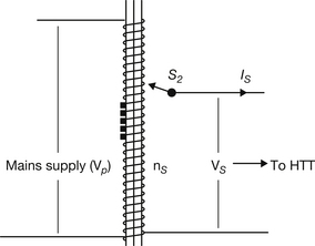
Figure 14.7 A circuit diagram for an autotransformer. It operates on the principle of self-induction. The number of secondary turn of the transformer can be varied at S2. Thus the output from transformer to the X-ray generator and high-tension transformer can be varied.
14.7.1 Losses and regulation in the autotransformer
All the sources of power loss discussed in Section 14.6 also apply to the autotransformer. However, the less severe design constraints required for the autotransformer make it possible to use a thick winding of copper wire with a consequent reduction in winding resistance. Therefore, the copper losses and the regulation are lower for the autotransformer than for the conventional transformer as both these losses are dependent on the resistance of the windings. One practical consequence of this is that there is not a great deal of heat generated in the autotransformer and so it is air-cooled.
14.8 The constant voltage transformer
Because it was manually operated the autotransformer has been replaced by the constant-voltage transformer. This will now be discussed in more detail.
The constant-voltage transformer is designed in such a way that there can be considerable variation in the input voltage to the transformer but the output voltage remains relatively constant. For reasons which will be discussed in Chapter 30, the output from the X-ray tube is sensitive to the temperature of the tube filament and so some units use a constant voltage transformer to ensure a well-stabilized voltage supply to the filament. Figure 14.8A gives a diagrammatic representation of the construction of such a transformer. Figure 14.8B shows a graph of the input and output voltages.
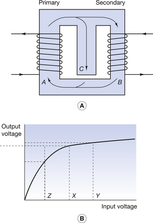
Figure 14.8 (A) Construction of a typical constant voltage transformer; (B) graph of the input and the output voltage for such a transformer.
This transformer operates on the principle that the secondary limb of the core, B, is magnetically saturated during normal operation. The magnetic flux produced at the primary core, A, passes through two other magnetic circuits, the much thinner secondary core, B, and a central path of high magnetic resistance in core C– this high magnetic resistance is caused by the fact that there is an air gap between one end of C and the rest of the core (remember, air is less permeable than iron). The thinner core, B, is rapidly brought to magnetic saturation and the excess magnetic flux then passes through C. As can be seen from the graph, once B is saturated then an increase in input voltage does not produce any more magnetic flux in B and so the output voltage from the transformer remains fairly constant. Magnetic saturation occurs at an input voltage of X, and Y on the graph represents the normal operating input voltage of the transformer. Note that a large fall in the input voltage (say to Z on the graph) can result in the limb B becoming unsaturated with a resultant fall in the output voltage.
14.9 Transformer rating
For transformer rating, the term rating means the maximum combination of factors that a system can withstand without damage. If the rating is exceeded for a transformer, this may cause damage to the electrical insulation of the windings because of overheating or it may cause electrical breakdown.
The transformers in an X-ray unit are energized when the X-ray exposure is made. There are basically two types of exposure in radiography:
1. Fluoroscopy – this uses a low amount of power for a relatively long time.
2. Radiographic exposures – these use a relatively large amount of power for a short time.
Each of the above produces heat in the high-tension transformer and this transformer thus requires oil cooling. In particular, a long exposure must be made at a relatively low current (and therefore low power), otherwise the heat generated in the transformer will not be convected away sufficiently quickly by the oil and the transformer will overheat. Short exposures may use higher current values since the total energy deposited in the windings will still be low enough to cause no damage.
The detailed specification of the rating of any one transformer may be complicated, dealing with all the conceivable situations in which the transformer may be used. There are three main factors that must be considered:
1. The maximum kVp that the secondary winding may produce.
2. The maximum continuous current the transformer may supply that would be used in fluoroscopy.
3. The maximum current supplied for short exposures – (that) would be used during radiographic exposures.
In this chapter, you should have learnt the following:
• The concept of an ideal transformer and the equations for voltage and current produced from such a transformer (see Sect. 14.3).
• How Faraday’s laws and Lenz’s law apply to transformers (see Sect. 14.4).
• The types of losses that occur in a practical transformer and how these are minimized (see Sect. 14.6).
• Transformer regulation and its effect on the output voltage from a transformer (see Sect. 14.6.3).
• The operating principles and main functions of an autotransformer in an X-ray set (see Sect. 14.7).
• The operating principles of a constant voltage transformer (see Sect. 14.8).
• The factors to be considered for transformer rating in radiography (see Sect. 14.9).