Chapter 20 The exponential law
Chapter contents
20.1 Aim 139
20.2 Description of the exponential law 139
20.3 Radioactive decay and the exponential law 140
20.4 Measures of radioactivity 141
20.5 Half-life and decay constant 142
20.6 Physical half-life, biological half-life and effective half-life 143
20.7 Attenuation of electromagnetic radiation by matter 144
20.8 Half-value thickness 145
20.9 Tenth-value thickness 146
20.10 The use of the exponential form of the logarithmic law 146
Further reading 147
20.1 Aim
The aim of this chapter is to introduce the exponential law and consider its applications to radiographic science. The law is fundamental to an understanding of radioactive decay and the attenuation of certain electromagnetic radiations (e.g. X-rays and gamma-rays).
20.2 Description of the exponential law
Perhaps the best everyday example of the exponential law concerns money. If £100 is invested with a financial institution which gives a fixed interest rate of 5% per annum then the growth of that money over a 25-year period is shown in Table 20.1 (See page 140).
Table 20.1 Growth of £100 at 5% per annum
| YEAR | INTEREST RATE (%) | MONEY AT END OF YEAR | NET INCREASE FOR YEAR |
|---|---|---|---|
| 1 | 5 | £105 | £5.00 |
| 2 | 5 | £110.25 | £5.25 |
| 3 | 5 | £115.76 | £5.51 |
| 4 | 5 | £121.55 | £5.79 |
| 5 | 5 | £127.63 | £6.08 |
| 6 | 5 | £134.01 | £6.38 |
| 7 | 5 | £140.71 | £6.70 |
| 8 | 5 | £147.74 | £7.03 |
| 9 | 5 | £155.13 | £7.39 |
| 10 | 5 | £162.90 | £7.77 |
| 11 | 5 | £171.03 | £8.13 |
| 12 | 5 | £179.59 | £8.56 |
| 13 | 5 | £188.56 | £8.97 |
| 14 | 5 | £197.99 | £9.43 |
| 15 | 5 | £207.89 | £9.90 |
| 16 | 5 | £218.29 | £10.40 |
| 17 | 5 | £229.90 | £10.91 |
| 18 | 5 | £240.66 | £11.46 |
| 19 | 5 | £252.70 | £12.04 |
| 20 | 5 | £265.33 | £12.63 |
| 21 | 5 | £278.60 | £13.27 |
| 22 | 5 | £292.53 | £13.93 |
| 23 | 5 | £307.15 | £14.62 |
| 24 | 5 | £322.51 | £15.36 |
| 25 | 5 | £338.64 | £16.13 |
Notice that the net increase per year is initially quite small (£5.00 in the first year) but the amount increases with time (£16.13 in the 25th year). This is an example of exponential growth in that as the time increases by equal amounts (1 year) the money increases by equal fractions (5%). If we draw a graph of the total money with the financial institution we get a smooth curve, as shown in Figure 20.1 (See page 140). This is the typical shape of an increasing exponential.
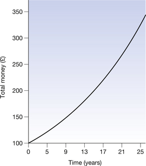
Figure 20.1 Growth of £100 at 5% per annum. Note that the rate of growth becomes greater with time. This is an example of exponential growth.
For a second example, consider a situation where we possess an initial sum of £100. If we consider a tax system where 5% of this money is removed each year as a tax, then the fate of the original £100 is shown in Table 20.2 (See page 141). Again we can note that the net decrease is greatest during the first year (£5.00) and is least during the 25th year (£1.46). The rate of decrease is, however, the same, at 5% per annum. This is an example of exponential decay in that as the time increases by equal amounts (1 year) the money left will decrease by 5% of that remaining, but will never reach zero (i.e. there will always be some money left). If we draw a graph of the total money left, we again get a smooth curve, as shown in Figure 20.2 (See page 141). This is the typical shape of a decaying exponential.
Table 20.2 Decrease of £100 at 5% per annum
| YEAR | TAX RATE (%) | MONEY AT END OF YEAR | NET DECREASE FOR YEAR |
|---|---|---|---|
| 1 | 5 | £95.00 | £5.00 |
| 2 | 5 | £90.25 | £4.75 |
| 3 | 5 | £85.74 | £4.51 |
| 4 | 5 | £81.45 | £4.29 |
| 5 | 5 | £77.38 | £4.07 |
| 6 | 5 | £73.51 | £3.87 |
| 7 | 5 | £69.83 | £3.68 |
| 8 | 5 | £66.34 | £3.49 |
| 9 | 5 | £63.02 | £3.32 |
| 10 | 5 | £59.87 | £3.15 |
| 11 | 5 | £56.88 | £2.99 |
| 12 | 5 | £54.04 | £2.84 |
| 13 | 5 | £51.33 | £2.70 |
| 14 | 5 | £48.77 | £2.57 |
| 15 | 5 | £46.33 | £2.44 |
| 16 | 5 | £44.01 | £2.32 |
| 17 | 5 | £41.81 | £2.20 |
| 18 | 5 | £39.72 | £2.09 |
| 19 | 5 | £37.74 | £1.99 |
| 20 | 5 | £35.85 | £1.89 |
| 21 | 5 | £34.06 | £1.79 |
| 22 | 5 | £32.35 | £1.70 |
| 23 | 5 | £30.74 | £1.62 |
| 24 | 5 | £29.20 | £1.54 |
| 25 | 5 | £27.74 | £1.46 |
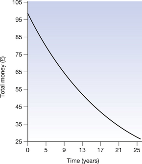
Figure 20.2 Decay of £100 at 5% tax per annum. Note that the rate of decay decreases with time and the amount of money left never reaches zero. This is an example of exponential decay.
The common factor in these two examples is that the change each year is 5%. This is characteristic of all exponential change and may be expressed as follows:
A quantity y is said to vary exponentially with x if equal changes in x produce equal fractional (or percentage) changes in y.
The two major examples of the exponential law in radiographic science are radioactive decay and the attenuation of electromagnetic radiation by matter. Both of these are described in the following sections.
20.3 Radioactive decay and the exponential law
Radionuclides are said to decay when they change from one nuclear configuration to another. This decay takes several forms, including the ejection of alpha-particles, beta-particles (both positive and negative) and gamma-rays from the nucleus. These and other modes of decay have been discussed more fully in Chapter 19. The particular mode of decay is, however, not important to our discussion in this section as the application of the exponential law is valid for all the modes. It can be stated as:
The law of radioactive decay states that the rate of decay of a particular nuclide (i.e. the number of nuclei decaying per second) is proportional to the number of such nuclei left in the sample (i.e. it is a fixed fraction of the number of nuclei left in the sample).
This is exactly analogous to the changes that occurred in the decaying exponential sum of money, in that a fixed fraction (or percentage) will decay each unit time (similar to the loss of money from the lump sum). Figure 20.3 shows a graph depicting the above situation. Note that the initial fall in number of atoms is steep but slows down as fewer and fewer of the original nuclei are left. Also note that the number of original nuclei never reaches zero. This is exactly the same as happened in the case of the lump sum of money and you should also note the similarities between Figure 20.3 (See page 141) and Figure 20.2.
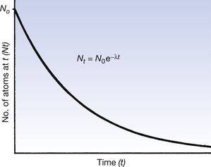
Figure 20.3 Exponential decay of the number of atoms of a particular radionuclide. (Note the similarity to Figure 19.2.)
20.4 Measures of radioactivity
In practice it would be extremely difficult to measure the number of nuclei remaining and draw a graph like Figure 20.3. What we can measure more easily is the effects of the nuclear disintegrations by counting the number of gamma-rays (for example) emitted, using a suitable counter. In this way we may make an estimate of the total number of disintegrations per second occurring within the radioactive sample at any given time. This quantity is known as the activity of the sample and is measured in becquerels, where 1 Bq is 1 nuclear disintegration per second. We may now plot activity against time (Fig. 20.4) and we obtain exactly the same curve as in Figure 20.3. The equation for this curve is expressed as:
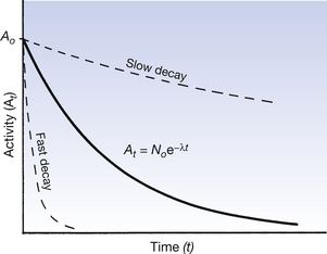

where At is the activity after a time t, A0 is the initial activity, e is the exponential constant, λ is the decay constant and t is the time after the initial measurement.
In practice it is often easier to use Equation 20.1 in its logarithmic form. (For more information on logarithms, see Appendix A.) Consider Equation 20.1:

If we take logarithms to the base e of both sides of the equation then we get:
This equation and its use with logarithmic graph paper will be considered further at the end of this chapter.
Figure 20.4 shows the decay curves for radionuclides which have different rates of decay. As we cannot consider the time it will take a nuclide to reach zero as a measure of its rate of decay, a quantity called the half-life is used to describe the rate of decay. This is further considered in the next section.
20.5 Half-life and decay constant
The half-life of a radionuclide is the time required for the activity of the radioactive sample to decay to one-half of its original value.
An illustration of the half-life of a particular radionuclide is shown in Figure 20.5 (See page 143). The activity of the sample when t=0 is A0. When the activity is reduced to A0/2 then the radionuclide has undergone one half-life. This is indicated by the time t1/2. If another half-life passes, then the activity is reduced by a further factor of 2 and is now A0/4, and so on for further half-lives. Notice that, as in our monetary example (Fig. 20.2), the curve never reaches zero activity, so no radioactive source is ever completely ‘dead’.
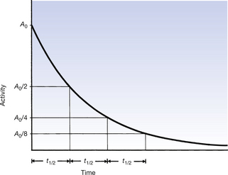
Figure 20.5 Half-life (t1/2) and the radioactive decay. Note that each t1/2 reduces the level of radioactivity by one-half.
If we now consider Equation 20.1, we can use this to establish a relationship between the decay constant and the half-life:

Now, by definition, at the half-life,  . Thus the equation can be rewritten in the form:
The decay constant is thus measured in time−1 since it is inversely related to the half-life. The decay constant is simply a constant of proportionality (see Appendix A).

Because of this relationship between the half-life and the decay constant, we may also write Equation 20.1 as follows:

Another important point is that it does not matter from which time measurement of the half-life is begun. Figure 20.6 (See page 143) shows the decay of a radionuclide over a time of one half-life starting from an arbitrary time, T. Note that the value of t1/2 shown in Figure 20.6 is exactly the same as the value shown in Figure 20.5. Thus, over an interval of t1/2 the activity is reduced by a factor of 2, independent of the starting time, T.
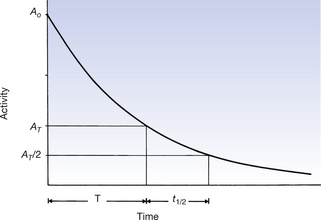
Figure 20.6 The half-life (t1/2) is measured from an arbitrary time, T. It is found that the value of t1/2 so obtained does not depend on the value of T, so the half-life may be measured from any starting time.
This example at the top of the next column gives some clue as to the general method of solving such problems. Assuming n half-lives of decay, the decayed activity An can be calculated from the formula:

where A0 is the original activity.
A radioisotope of iodine, 131I, has a half-life of 8 days. Its activity was measured as 14.4 MBq at 09:00 on 3 February. What will be its activity at 09:00 on 27 February?
The time interval over which we are considering the decay of the nuclide is 24 days. With a half-life of 8 days, this represents decay through three half-lives.
After one half-life the activity will be reduced by a factor of 2.
After two half-lives the activity will be reduced by a factor of (2 × 2)=4.
After three half-lives the activity will be reduced by a factor of (4 × 2)=8.
So each successive half-life reduces the activity by a factor of 2.
Thus the activity after three half-lives=14.4/8=1.18 MBq.
The activity at 09:00 on 27 February will therefore be 1.18 MBq.
Similarly, we can use this equation to look back to consider how much original activity would be required on a certain date to give us the required activity at the time of use of the isotope. Here the unknown is A0 and the equation can be rearranged as follows:

An activity of 36.5 MBq of 99Tcm is required at 17:00 on 22 March. The radionuclide has a half-life of 6 h. What activity of the isotope must be dispensed at 05:00 on 22 March to give the required activity?
Using Equation 20.6:
20.6 Physical half-life, biological half-life and effective half-life
In all the considerations of radioactive decay so far we have considered the physical half-life of an isotope – the half-life as it would be measured using a quantity of isotope in the laboratory. In nuclear medicine there are two other types of half-life we need to consider:
1. The biological half-life is the time taken for the concentration of a certain chemical in an organ to be reduced to half its original concentration. In this case, the concentration of the chemical is the important part and its activity is not important. This value is affected by the body’s ability to excrete the chemical.
2. The effective half-life is the time taken for the activity of a certain radionuclide in a certain organ to be reduced to half of its original activity. This will be affected by the physical half-life and the biological half-life.
The three types of half-life are connected by the equation:
20.7 Attenuation of electromagnetic radiation by matter
The attenuation of electromagnetic radiation by matter constitutes the other major application of the exponential law in radiography.
The types of interactions which electromagnetic radiation undergoes when it passes through matter are explained in Chapter 23. A detailed knowledge of these mechanisms is not required at this stage. If we consider a slab of material which has 100 units of radiation incident on it and the transmitted radiation measures 90 units, then we can say that the material attenuates 10 units of radiation (the differences between absorption and attenuation will be explained in Ch. 23).
For the exponential law to be applied, certain conditions must be satisfied:
• The radiation beam must be parallel. This means that it is not affected by the inverse square law.
• The radiation beam must be homogeneous (i.e. the photons must all have the same energy). This means that the beam is not ‘hardened’ by the removal of low-energy photons by the attenuating material.
• The attenuator must be homogeneous. This means that the attenuating properties must be the same in different parts of the attenuator.
Consider the situation in Figure 20.7. Here, a parallel beam of radiation (e.g. gamma-rays) is incident on a slab of uniform attenuating material of thickness x. Suppose there is 10% attenuation in the first slab, then 90% of the original beam is transmitted. If we put a further identical attenuator in the path of the beam, then it is found that it also attenuates 10% of the radiation incident upon it and 81% (0.9 × 90%) will be transmitted. A third identical attenuator transmits 90% of this amount (72.9%), and so on for further attenuators. From this we can say that equal changes in x produce equal fractional (or percentage) changes in the transmitted radiation intensity. This is again an exponential relationship, so we can say that:
The attenuation of a monoenergetic parallel beam of electromagnetic radiation by a uniform attenuator will vary exponentially with the attenuator thickness.
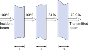
Figure 20.7 Exponential attenuation of a parallel beam of electromagnetic radiation by matter. Equal thickness (x) of the attenuator will transmit equal fractions (in this case 9/10) of the incident radiation.
A graph of the transmitted intensity Ix through the attenuator of thickness x is shown in Figure 20.8. The incident radiation I0 is the value of Ix when there is no attenuator (x=0). Note the similarities between this curve and the other exponential curves shown in this chapter. The mathematical relationships between the quantities can be given using equation:
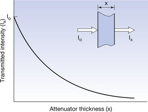
Figure 20.8 Graph showing changes in transmitted intensity due to exponential attenuation of radiation by a uniform attenuator. Note the similarity to Figure 20.3.

where μ (mu) is the total linear attenuation coefficient and so takes into account all the processes of attenuation. The equation therefore refers to variations of transmittance within linear distance, x.
20.8 Half-value thickness
If we consider Figure 20.9, we can see that successive half-value thicknesses (HVTs) reduce the intensity by factors of 2, and are therefore in a position to define HVT more precisely.
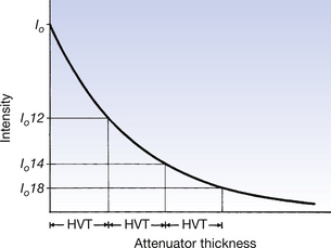
Figure 20.9 Half-value thicknesses (HVT) of a beam of electromagnetic radiation. Each HVT of the attenuator reduces the intensity by one-half. Note the similarity to Figure 20.5.
The half-value thickness is that thickness of a substance which will transmit one-half of the intensity of radiation incident upon it.
The HVT therefore depends on the attenuating properties of the substance itself and the penetrating power of the beam of electromagnetic radiation incident upon it. In diagnostic radiography, we might compare the penetrating properties of two beams using aluminium to the HVTs, whereas in therapeutic radiography we would do this using copper as our attenuator. This is because the photon energy is higher in therapeutic radiography so we need to use a material with a higher atomic number.
To complete the analogy with radioactive decay, Equation 20.3 is paralleled by:

a. The HVT for a beam of radiation is found to be 2.8 mm of aluminium. What is the total linear attenuation coefficient of this beam in aluminium?
From Equation 20.9:

b. The HVT for a particular beam of gamma-rays is 3 mm of lead. What thickness of lead must be placed in the beam such that only 0.1% of it is transmitted?
There are several ways of tackling this and similar problems. Below is one method.
One-hundred per cent of the beam is incident on the lead and 0.1 % is transmitted. This gives a reduction factor of 100/0.1=1000.
Now each HVT gives a reduction factor of 2 between the incident and the transmitted radiation, as shown in the table below:
| NUMBER OF HVTS | INTENSITY REDUCTION FACTOR |
|---|---|
| 1 | 2 |
| 2 | 4 (i.e. 2 × 2) |
| 3 | 8 |
| 4 | 16 |
| 5 | 32 |
| 6 | 64 |
| 7 | 128 |
| 8 | 256 |
| 9 | 512 |
| 10 | 1024 |
This sort of table is very easy to check so there should be little chance of arithmetic errors.
After 10 HVTs, the intensity reduction factor is 1024, which is very close to the required factor of 1000.
Thus, 30 mm of lead (10 HVTs) must be used to reduce the transmitted intensity to 0.1% of the incident intensity.
As was the case with radioactive decay (see Equation 20.5), we can use a formula to calculate the intensity (In) after n HVTs:

20.9 Tenth-value thickness
It should be clear at this stage that values of absorber thickness other than the HVT will produce equal fractional changes in transmission and so it is possible to define a ‘fifth-value thickness’ or a ‘tenth-value thickness’ (TVT), etc. Although the HVT is a very common method of measuring the attenuation of electromagnetic radiation through matter, the TVT is also used when considering large amounts of attenuation. An example of this would be when designing the walls of a radiotherapy treatment room when a very high intensity of radiation from the treatment machine must not be allowed to penetrate through the wall in significant quantities. One TVT would reduce the intensity by a factor of 10; two would reduce the intensity by a factor of 100, and so on.
20.10 Use of logarithmic form of the exponential law
Consider Equation 20.2, which is the logarithmic form of the exponential law:
If we look at this equation, we see that it is in the form of y=c − mx and so we would expect its graph to be in the form of a straight line. If we plot loge of the activity on the y-axis and time on the x-axis, we get the graph shown in Figure 20.10.
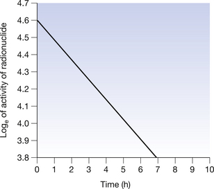
Figure 20.10 Graph of the logarithm to the base e of the activity of a radionuclide plotted against time. Note that the previous exponential curve (see Fig. 20.4) is now a straight line.
The requirement to calculate the logarithm for each result and the antilogarithm for each reading from the graph is overcome by the use of logarithmic graph paper (for a fuller description, see Appendix A). Suitable graph paper in this case is log/linear graph paper, i.e. the y-axis is logarithmic and the x-axis is linear.
An example of such a graph for the attenuation of a beam of electromagnetic radiation is shown in Figure 20.11. Note that equal spaces on the log scale represent changes by factors of 10, and so the logarithmic scale never reaches zero. This type of paper allows us to plot the points directly on the paper and then draw the best straight line through them. Such a linear graph makes it easier to interpolate and to extrapolate (see Appendix A) information from the graph.
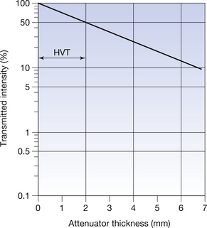
Figure 20.11 An example of the use of logarithmic graph paper to plot an exponential relationship. Note that the previous exponential curve (Fig. 20.8) has now has become a straight line. The half-value thickness (HVT) for the beam of radiation is 2 mm, as read from the graph. Half lives may also be determined in the same manner.
In this chapter, we have considered the following factors pertinent to the exponential law:
• The description of the exponential law (see Sect. 20.2).
• Radioactive decay and the exponential law (see Sect. 20.3).
• Measures which can be made of the activity of a radionuclide (see Sect. 20.4).
• The relationship between the half-life and the decay constant for a radionuclide (see Sect. 20.5).
• The relationships between the physical half-life, the biological half-life and the effective half-life (see Sect. 20.6).
• How the attenuation of electromagnetic radiation by matter obeys the exponential law (see Sect. 20.7).
• The HVT for a beam of radiation and a given attenuator (see Sect. 20.8).
• The use of the TVT (see Sect. 20.9).
• The use of the logarithmic form of the exponential law (see Sect. 20.10).
Further reading
Radioactivity and the exponential law
Chapter 19 of the current text contains more information on this topic.
Ball J.L., Moore A.D., Turner S. Ball and Moore’s Essential Physics for Radiographers, fourth ed. London: Blackwell Scientific, 2008. (Chapter 20)
Dendy P.P., Heaton B. Physics for Diagnostic Radiology. Institute of Physics, second ed. 1999. (Chapter 1)
Webb S., editor. The Physics of Medical Imaging, second ed., Bristol: Institute of Physics, 2000. (Chapter 6)
Exponential attenuation of radiation
Ball J.L., Moore A.D., Turner S. Ball and Moore’s Essential Physics for Radiographers, fourth ed. London: Blackwell Scientific, 2008. (Chapter 17)
Bushong S.C. Radiologic Science for Technologists: Physics, Biology and Protection, ninth ed. New York: Mosby, 2009. (Chapter 4)
Dendy P.P., Heaton B. Physics for Diagnostic Radiology. Institute of Physics, second ed. 1999. (Chapter 3)