Appendix A Mathematics for radiography
Chapter contents
A.1 Algebraic symbols 329
A.2 Fractions and percentages 330
A.3 Multiplying and dividing 331
A.4 Solving equations 332
A.5 Powers (Indices) 334
A.6 Powers of 10 335
A.7 Proportionality 336
A.8 Graphs 336
A.9 The geometry of triangles 338
A.10 Pocket calculators and calculations in examinations 339
A.11 Logarithms 339
A.12 Vector quantities 340
Answers to exercises 340
This appendix on the revision of mathematics is directed primarily at those whose mathematics is a little weak. However, many of the worked examples shown are chosen from topics in radiography.
For those studying for examinations, the following remarks may be of help. Examiners frequently complain of cramped, untidy mathematics which is difficult to follow. What they are hoping to see in the answer is a clear statement of the problem and an easy-to-follow development of the mathematics used to obtain the solution. This may be more important (and hence gain more marks) than simply obtaining the correct numerical answer. In fact, the correct answer simply recorded on its own with little or no supporting mathematical reasoning will not achieve many marks – remember that the examiner cannot know how you achieved the final answer unless you tell him/her. In practice, you should use phrases and sentences to tell the examiner how you have progressed from one step of the problem to the next as you move towards the eventual solution. This should also help you to think more clearly about what you are doing and also to check the integrity of your final answer – this is probably even more important with the widespread use of pocket calculators. A study of the worked examples in this appendix should clarify these points.
A.1 Algebraic symbols
The letters of the English and Greek alphabet (see Table D following the appendices) are often used to represent the magnitude of an unknown quantity. For example, an electrical potential difference may be represented by V volts, an angle by θ (i.e. theta) degrees or radians and an energy by E joules. Such a practice enables the symbols to be used in place of the actual numerical values of the quantities, and is of great practical use in solving equations (see App. A.4).
A.1.1 Suffixes
Suffixes are used to denote a specific value of a particular quantity. If we use the symbol I to denote the intensity of radiation from a particular source, then I will depend upon the distance from the source at which the intensity is measured (see Ch. 26). We may call a particular distance x, say, and denote the intensity of this distance by Ix – meaning the intensity at x. For another distance y, the corresponding value of intensity is Iy.
Similarly, if a quantity, N, changes with time, t, the value of N at any given time may be denoted by Nt.
Suffixes are used, then, to avoid ambiguity and are used as such in many chapters of this book.
A.2 Fractions and percentages
Although fractions are not commonly used in radiographic calculations since they have been largely replaced with decimals, nevertheless a knowledge of how to manipulate fractions mathematically is useful in calculations involving Ohm’s law (see Ch. 7) and capacitors (see Ch. 13). For this reason, a section on fractions and percentages is still included in this appendix.
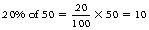
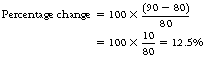
A.2.1 Percentages
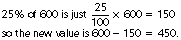
If a quantity increases in value by 50 per cent (%), then this means that it has become greater by one-half of its previous value. Thus, if the electric current passing through an X-ray tube was 200 mA, then an increase of 50% would bring this to 300 mA. Alternatively, it may be said that the new value is 150% of the original value.
In general terms, if a is the original value of a quantity and b is its new value, then:
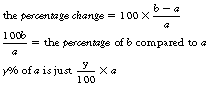

A percentage is a special case of a fraction, where one number is divided by another. The following sections describe how fractions may be added together and multiplied.
A.2.2 Addition of fractions
Suppose we have the fraction a/b, where a and b represent general numbers. Now the addition or subtraction of a/b to another fraction c/d rests on the fact that we can take any fraction and multiply top and bottom by the same factor (k, say) without altering its value:
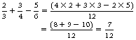
It is the appropriate selection of k for each fraction which makes for the easy addition of fractions. For example, suppose we have:

If we multiply 2/3 by 2 (top and bottom), we shall have a fraction expressed in sixths, just like the second fraction:
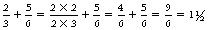
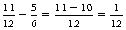
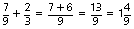
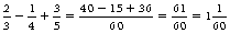
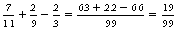
Notice that we multiplied only the first fraction – we need not do the same thing to the second. This method is often very quick, particularly when only two or three simple fractions are involved, and is in fact entirely equivalent to the more general method of using the lowest common denominator (LCD), as illustrated in the following example:
Here, the LCD of the denominators 3, 4 and 6 is 12 and is therefore used as the overall denominator on the right-hand side. The individual denominators are then divided into 12, the result being multiplied by the respective numerator and summed (observing the correct signs) as shown in the example.


A.3 Multiplying and dividing
A.3.1 Positive and negative numbers
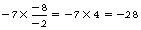
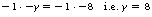
It is obvious that 1×8=8, but what are −1×8, −1×−8 and 8×–1?
To avoid having to work out such problems from first principles every time, a simple rule has been developed which we may call Rule 1.
i.e. only when the signs are dissimilar is the result negative.


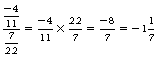
A.3.2 Fractions
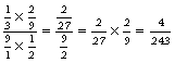
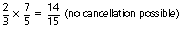
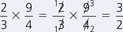
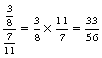
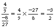
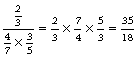
The multiplication of two or more fractions is just a matter of simplification by cancellation (where possible) and then multiplying all the numerators together to form the new numerator, and all the denominators together to form the new denominator.
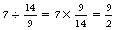
The division of two fractions is straightforward provided that the following rule is obeyed.
Let us say, by way of illustration, that we wish to divide 4 by ½:

Applying Rule 2, we turn ½ upside down and multiply:

Is this the answer we would expect intuitively? Well, the problem may be expressed as ‘how many halves are there in 4?’, and then it is obvious that the answer is 8. Some more examples to clarify the method:


A.3.3 Brackets
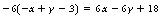
A bracket links two or more quantities together such that the bracket and its contents may be treated mathematically as a single quantity. If we wish to remove the brackets, then care over the plus and minus signs must be taken (Rule 1).
Multiplying two or more brackets together can become quite involved. However, it is rare for problems in radiography to require even the multiplication of two brackets, but the method is outlined below for the sake of completeness.
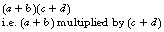
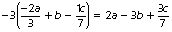
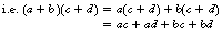
To perform this calculation, we take the first term of the first bracket, a, and multiply it by (c + d). Then we add the result to the multiplication of the second term, b, by (c + d):
Again, we must be careful of the sign convention (Rule 1), as the following two worked examples show.
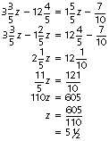
A.4 Solving equations
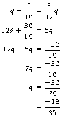
Many of the types of equations encountered in problems associated with radiography are those in which a single ‘unknown’ (whose numerical value we wish to calculate) is ‘mixed up’ with several other numbers which may occur on both sides of the equation. (The solution of several equations involving several unknowns, i.e. simultaneous equations, is not normally required, and so will not be discussed here.) Our task, then, in the equations encountered, is to ‘unscramble’ the unknown so as to leave it on one side of the equation and all the numbers on the other side – the equation is then said to be ‘solved’. This process is straightforward, provided that the following simple rule is obeyed:
This rule is intuitively obvious if it is imagined that the equals sign of the equation is the pivot of a pair of scales which is in exact balance. Whatever weight we now add to or subtract from one scale-pan must be added to or subtracted from the other or the scales will no longer be in balance. Similarly, if we double (say) the weight on one side we must do the same to the other – thus, provided we multiply by the same factor, balance is preserved and one side is equal to the other side. For example, consider the simple equation:

If we add 2 to the left-hand side (LHS) of this equation the −2 will be cancelled, leaving x only. However, in accordance with Rule 3 above, we must add 2 to the right-hand side (RHS) in order to preserve equality:

Putting x=5 in the original equation, we have 5−2=3, which is correct.
As another example, consider: 15−y=7. Subtracting 15 from both sides so as to eliminate it from the LHS:

Multiplying both sides by −1 in order to make both terms positive (Rule 1), we have:
(Note: The symbol ‘.’ is often used, as above, to denote multiplication.)
Substituting our solution into the original equation to serve as a check, as in the previous example, we have:

thus verifying our answer.
It is apparent from these examples that a convenient way of picturing this type of mathematical operation is that of ‘transferring a quantity from one side to the other and changing its sign’. Obviously, this only applies to the elimination of variables by addition or subtraction, not multiplication, which will be discussed in the next example.


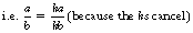
This last step is known as cross-multiplication and may be pictured in the following manner:
 (cross-multiplication)
The double-ended arrows indicate that movement may be in either direction. Note that there is no change of sign.
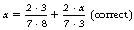
One incorrect use of cross-multiplication occurs so frequently that it is worth a special mention here. Suppose we have the equation:

if we cross-multiply in the following manner:
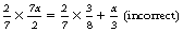
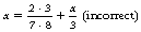
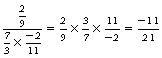
The fault lies, of course, in the fact that Rule 3 has been disobeyed, i.e. the term x/3 remains unaltered although we were intending, by our cross-multiplication, to multiply both sides by 2/7. Hence, if we wished to cross-multiply at this stage, we should have obtained:


A.5 Powers (Indices)
An index is written at the top right of a quantity (the base) and refers to the number of times the quantity is multiplied by itself. For example, 53 means 5×5×5 (i.e. 125). It is a convenient mathematical ‘shorthand’ to write powers of a number in this way. In this example, the index is a positive integer (i.e. 3), but this need not be the case for it may be positive, negative, fractional or decimal, as described below.
A.5.1 Combining indices
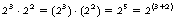
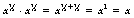
Let us assume that we have two numbers, 23 and 22, which we wish to combine by addition, multiplication and division in order to elicit general rules for the handling of indices.
A.5.1.1 Addition
Using the definition of an index as described above:

Thus, when adding such numbers, each term is calculated separately prior to addition (or subtraction).
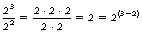
A.5.2 Negative indices
Suppose that we wish to divide 42 by 44. From first principles (Sect. A.5), we have:
Also, by the rule on division as described above, we may subtract indices:

Since equations (A.1) and (A.2) are equal:


i.e. to change a negative index to a positive index, just take the reciprocal, as shown in Equation A.3.

A.5.3 Fractional indices

from the definition of a square root.
Thus, from inspection of these two equations:


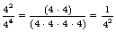
A.5.4 The zero index – x0
A general number x raised to a power m is xm. If we divide xm by itself, the answer will obviously be 1. But xm÷xm is xm−m by the rules discussed above. Thus 1=xm−m=x0. Since we took any general number, this result is also general (except for 00, which is indeterminate).
A.5.5 Indices to different bases
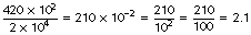
A problem on the inverse square law (see Ch. 26) frequently involves calculation of the form:

Here a, b and c represent numbers whose values are known, having been specified by the problem. We wish to determine the best way of obtaining the final result, since b and c are frequently large numbers, whose squares are therefore even larger. This means that the probability of making an arithmetical error can be quite high if a laborious method of calculation is undertaken. However, a great simplification is possible if we remember that:

If b=90 cm and c=60 cm then b2/c2 the ‘hard’ way is:
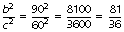
which may be cancelled to give 2.25 – this exercise being left to the reader. The ‘easy’ way is to use Equation A.4, i.e.:
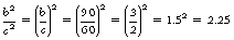
Note that the answers are the same, as we should expect, but that the second method involves cancelling of smaller numbers so that there is less likelihood of an arithmetical error.
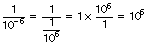
A.6 Powers of 10
When 10 is used as a base for indices, all the findings of the previous section apply. In addition, powers of 10 are very useful when measuring very large or very small quantities of a given unit, as shown in Table A.1.
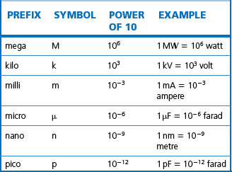
Other names not shown in the table exist (see Table A after the appendices), but these are all that we shall need. It is advisable for the student to memorize these terms as they are in very common usage in radiography. The following exercise is included for this purpose.
a. An X-ray tube has a current of 0.05 amperes passing through it. How many milliamperes (mA) does this correspond to?
b. If the X-ray tube has a peak potential difference of 125 000 volts across it, what is the value in kilovolts (kVp)?
c. Express a capacitance of 0.000 065 farads in microfarads (μF).
d. A photon of light has a wavelength of 550 nanometres (nm). What is this in metres?
A.7 Proportionality
A.7.1 Direct proportion
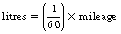
If a car is travelling at constant speed such that the petrol consumption is a steady 60 km.l−1, then:
Thus, the amount of petrol consumed is in direct proportion to the number of miles travelled, and we may write:

where the sign ‘∝’ means ‘is proportional to’. Alternatively, we may write:
In general, therefore, if two quantities y and x are directly proportional to each other, then:

where k is called the ‘constant of proportionality’. Some examples of direct proportionality which are discussed in the main text include the following:
A.7.2 Inverse proportion
Suppose that we have many rectangles of equal area, k, but of differing heights (h) and widths (w). However, in each case the area is the same, so that:

Then, since k is constant, we may write:

In this case, therefore, h and w are in inverse proportion, since w is halved if h is doubled, and vice versa. This is opposite to direct proportion, of course, where doubling (say) one quantity also doubles the other.
Examples of inverse proportion discussed in the main text include:
• The capacity (C) of a parallel-plate capacitor is inversely proportional to the separation (d) between its plates, i.e. C ∝ 1/d (Ch. 13).
• The intensity (I) from a point source of electromagnetic radiation is inversely proportional to the square of the distance (x) from the source, i.e. I ∝ 1/x2 (Ch. 26).
• The electrical resistant (R) of a given length of wire varies inversely as the area of cross-section (A), i.e. R ∝ 1/A (Ch. 7).
A.8 Graphs
A.8.1 Drawing and interpretation
A good understanding of the construction and interpretation of graphs is of great value in radiography, radiotherapy and nuclear medicine. The following simple but effective rules are offered in the drawing of good graphs:
• Each graph should take at least one-third of a page – use as large a scale as practicable so that you can make accurate readings.
• Each graph should have a clear, appropriate title.
• The axes, which should be drawn with a ruler, should be of approximately equal length.
• Both axes must be clearly labelled to show what is being measured and should contain units (cm, s, kg, etc.) where appropriate.
• The independent variable is normally on the x-axis, and the dependent variable on the y-axis, i.e. the variable which is being measured is plotted on the y-axis while the variable causing the change in y is plotted on the x-axis. If we consider plotting the radioactivity from a sample over a period of time, then the independent variable is time (plotted on the x-axis) while the dependent variable is the radioactivity (plotted on the y-axis).
The following examples have been chosen to illustrate both the drawing and the interpretation of graphs.
As described in the last section, two quantities, x and y, are directly proportional to each other if y=kx, where k is a constant. Figure A.1 shows y=kx in graphical form.
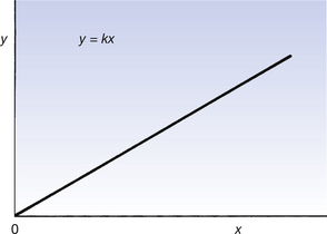
The following points should be noted:
• The graph passes through the origin, since when x=0, y is also equal to zero.
• The slope (or gradient) of the straight line produced is a measure of how steep it is and is defined as the change in y divided by the corresponding change in x. Since the graph passes through the origin, this is a convenient place from which to measure the changes. From this it can be seen that the slope is y/x. But from the equation y=kx it can be seen that y/x=k. Thus the slope increases as k increases.
• The general equation for a straight line will be in the form y=mx+c where m is the gradient of the line and c is the intersection of the line with the y-axis – the value of x when y=0.
Example 2 – Inverse proportion
Figure A.2 shows a graph of the inverse relationship between the capacitance, C, of a parallel-plate capacitor and the distance of separation of its plates, d, where C ∝ 1/d or C=k/d for a specific capacitor.
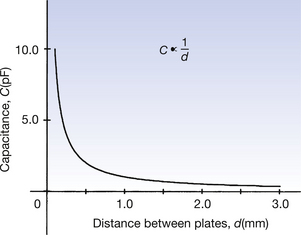
From the graph it can be seen that as the distance between the plates increases, so the capacitance of the capacitor decreases.
Rating charts are supplied by the manufacturers of X-ray tubes, and contain a lot of information in graphical form which is an essential guide to the radiographer in the selection of ‘safe’ exposure factors, i.e. the combination of focal-spot size, kVp, mA and exposure time which will not cause damage to the X-ray tube.
An example of a rating chart is given by Figure A.3, where a family of curves represent the maximum permissible exposure factors for different settings of kVp. The use of rating graphs is discussed in detail in Chapter 31 and we only need to make the point here that points below a particular curve for one kVp setting are ‘safe’, while points above it lead to tube damage by overheating the anode.
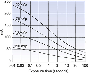
Note the non-linear (logarithmic) scale on the x-axis. Logarithmic scales are discussed in Chapter 20.
A.8.2 Interpolation and extrapolation
It is often the case that a graph is drawn using a relatively small number of points, and that these points are joined together with a curve or straight line passing through them. The smooth curve or line makes it possible to ‘read off’ values from the graph, even when such values lie between the original points used to construct the graph. This procedure is known as interpolation and is one of the advantages of the graphical method.
If it is desired to determine the value of one of the plotted variables when it lies outside the range of the points used to plot the graph, the curve may be extended, or extrapolated, to reach this region. However, such an extrapolation can lead to large inaccuracies, since several different curves may seem equally suitable and there may be no way of knowing which one is correct!
a. Draw a graph of y=0.2x, choosing values of x from 1 to 10 in steps of 1. Hence read from the graph the value of y when x is (i) 1.5, (ii) 9.5, (iii) 12, (iv) 0.5. Verify your answers by substitution into the original equation.
b. Repeat the same procedure for the equation y=0.2x2. (Note the increased uncertainty in obtaining the extrapolated value of y when x=12.)
A.9 The geometry of triangles
A.9.1 The right-angled triangle
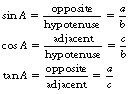
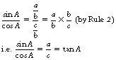
Consider the right-angled triangle shown in Figure A.4. The trigonometric functions of sine, cosine and tangent are defined as:
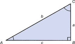
Figure A.4 A right-angled triangle. See text for definition of sine, cosine and tangent of an angle.
a. Write down expressions for sin C, cos C and tan C from Figure A.4.
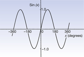
The sine function occurs frequently throughout this book, e.g. in the geometry of triangles and in alternating current theory (Ch. 11). Its graphical form is shown in Figure A.5. This graph is known as a ‘sine wave’, and always lies between +1 and −1. Also, the shape of the curve is cyclical, repeating itself every 360°.
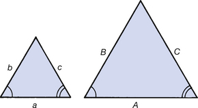
A.9.2 Similarity of triangles
The two triangles shown in Figure A.6 are said to be ‘similar’ because one is just a bigger version of the other, while retaining the same shape. Thus, the corresponding angles of the two triangles are equal, but the lengths of the corresponding sides need not necessarily be so. However, if one side has a length which is double (say) that of the corresponding side of the other triangle, than all the sides will be doubled compared to the other triangle. Generally, then, we may write:

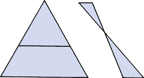
In many practical examples in radiography, however, the similar triangles look more like those shown in Figure A.7.
A.10 Pocket calculators and calculations in examinations
Because the price of pocket calculators now puts them within the range of even the most impoverished student, the purchase of such a calculator is strongly recommended. ‘Scientific’ pocket calculators have the advantage that they can perform calculations which involve trigonometrical and logarithmic functions and so will be found especially useful. Many such calculators are also ‘programmable’ which means that formulae may be inserted into the calculator memory to allow it to perform certain calculations by simply inserting the appropriate data – a formula for Ohm’s law could be inserted so that when the program is invoked the calculator will automatically calculate the resistance from the value of the potential and the current.
If you are to use a pocket calculator in examinations or if you are about to buy one, here are some suggestions which you might find helpful:
• Consider the types of calculations which you require from the calculator and do not buy one with lots of unnecessary functions – these simply increase your chance of error.
• Try out a calculator before you buy it (if possible) and, if you are about to use one in an examination, make sure you are familiar with its layout and functions.
• Find out the policy regarding the use of calculators in examinations at your university. Some universities will issue calculators for the purpose of examinations while others have specific regulations regarding programmable calculators.
• Remember that the calculator will only give the correct answer if the correct information is keyed into it. It is important to remember indices and also try to get some ‘feel’ for the magnitude of the correct answer.
A.11 Logarithms
Although few students would now undertake calculations using logarithms as the chosen method – thanks to the ease of use of the pocket calculator – it is nevertheless helpful to have a basic grasp of the theory of logarithms to explain certain functions in radiography, e.g. it may be easier to understand the exponential equations (see Ch. 20) in their logarithmic form.
The logarithm of a number to a given base is the power by which the base must be raised to give the number.
Thus, the logarithm of 100 to the base 10 is 2 as 102=100. This would normally be written as log10100=2.
The base can be any number but, in practice, logarithms are usually to the base 10 or to the base e where e is the exponential number and is approximately equal to 2.7183.
Consider a situation where we wish to multiply two numbers a and b. If a=10x and b=10y then:

Thus, from our initial definition of logarithms we can say:

By a similar argument it can be shown that:
The main use of logarithms in radiography is to allow the simplification of complex formulae – if we consider the intensity of a beam of radiation which has travelled a distance x through a medium, this is given by the equation:

where Ix is the intensity of the radiation after a thickness x, I0 is the initial intensity of the radiation, e is the exponential number and μ is the linear attenuation coefficient – these are all explained in Chapter 20. This equation is quite complicated to use in the above form but is much easier to use in its logarithmic form:

A.12 Vector quantities
In vector quantities, the quantity concerned has direction as well as dimension. Thus, in vector addition we need to take both these factors into account. This is probably best illustrated by two simple examples:
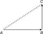
1. A man walks 30 metres in an easterly direction and then walks 20 metres in a northerly direction. How far must he walk in a straight line to get back to where he started? The situation may be visualized using Figure A.8. By applying Pythagoras’ theorem to this we can calculate that the distance from C to A is 36 metres.
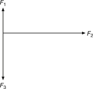
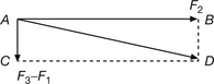
2. Forces F1=1 newton, F2=4 newtons and F3=2 newtons are applied to a point source as shown in Figure A.9. What is the resultant force and what is its direction? As F1 and F3 are in opposite directions, the resultant force is the difference between F1 and F3 and is in the direction of F3 as this is the larger of the two forces. We can now do vector addition (see Fig. A.10), where AB represents force F2 and BD represents (F3 − F1). The resultant force is represented by AD. By application of Pythagoras’ theorem, the length of this line is 4.12 newtons. Tan A is BD/AB and thus A can be calculated as approximately 14°. Thus we can say that the resultant force measures 4.12 newtons and is in a direction 14° below the horizontal.
• If we multiply or divide two +s or two −s, we get a +.
• If we multiply or divide a + and a − sign, we get a −.
• When dividing by a fraction, we can get the same result if we multiply by the fraction inverted (the fraction turned upside down).
• The following mathematical relationships have been established:
• In direct proportion, y ∝ x or y=kx while in inverse proportion, y ∝ 1/x or y=c/x where k and c are constants of proportionality.
• Sin θ=opposite/hypotenuse; cos θ=adjacent/hypotenuse and tan θ=opposite/adjacent.
• Sine and cosine functions are cyclical, repeating themselves every 360°.
• When drawing graphs, use a manageable scale, use a ruler, label both axes and use a title.
• Similar triangles have the ratio of their corresponding sides equal.
• There are certain factors to consider when purchasing or using a pocket calculator.
• The basic theory of logarithms tells us that if y=xn then logxy=n.
• In vector addition, we can get the resultant vector by joining the vectors end to end. The resultant vector is from the origin to the tip of the last vector.