Chapter 25 The radiographic image
Chapter contents
25.1 Aim
The aim of this chapter is to consider the major factors involved in the production of a radiographic image. The chapter will first consider the attenuation patterns in a patient that will produce an X-ray image and will then consider how this reacts with a recording medium to produce a radiograph. The chapter also summarizes how the selection of exposure factors affects the quality of the radiographic image produced.
25.2 Introduction
The quality of the radiographic image is affected by a number of geometrical factors that determine the magnification of the image and the amount of geometrical unsharpness produced. The radiographic image depends on more than geometrical considerations. This chapter considers the other factors which contribute to the image quality. To understand this, it is necessary to understand the contribution of photoelectric absorption and Compton scattering to the final radiographic image (see Ch. 23).
It is easier to understand the final image quality if we consider image formation as a two-stage process:
1. The production of an X-ray image pattern as the beam of radiation is attenuated by the patient.
2. The production of a radiographic image as this radiation pattern interacts with a recording medium.
Therefore, this chapter will consist of two halves, each looking at one of these stages.
25.3 The X-ray image pattern
25.3.1 Attenuation of the X-ray beam by the body
We will assume, for simplicity, that the radiation beam from the X-ray tube striking the body is of uniform intensity across the beam. When this beam interacts with the body substance, different structures will cause different amounts of attenuation and a ‘pattern’ of radiation intensities is transmitted to the imaging device. If all structures in the beam attenuated the radiation by the same amount, there would be no pattern and no image of any structures would be seen on the radiograph. A simple example of such differential absorption is shown in Figure 25.1, where two separate rectangular blocks of bone and soft tissue are shown interacting with the X-ray beam. The profiles of the incident (I0) and the transmitted (IT) radiation intensifies are also shown. If again we assume, for simplicity, that the attenuation of the radiation beam is exponential, then:
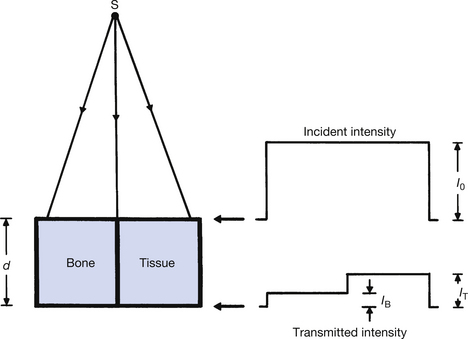
Figure 25.1 A comparison of the attenuation of an X-ray beam by an equal thickness of bone and soft tissue. Note that the attenuation of X-rays by bone is greater than that by soft tissue.

where I0 is the intensity of the X-ray beam before it enters the patient, μ(B) is the total linear attenuation coefficient for bone and μ(T) is the total linear attenuation coefficient for soft tissue. IB is the intensity of the radiation transmitted through a thickness d of bone and IT is the intensity transmitted through a similar thickness of soft tissue. As can be seen from Figure 25.1, IB is less than IT. This is because μ(B) is greater than μ(T). There are two physical reasons for this:
1. The density of bone is approximately twice that of soft tissue (ρB=1.8; ρT=1.0).
2. The average atomic number of bone is approximately twice that of soft tissue (ZB=14; ZT=7.5).
The total linear attenuation coefficient is proportional to the number of atoms present in unit volume and the density of the medium. As the density of bone is twice that of soft tissue, then there must be twice as many atoms in unit volume and so, all other things being equal, the linear attenuation coefficient for bone would be twice that for soft tissue.
To appreciate the importance of the difference in atomic number, we must consider the attenuation process occurring. The equations for each process are summarized below:
where τ is the linear attenuation coefficient for the photoelectric effect, σ is the linear attenuation coefficient for Compton scattering, ρ is the density of the attenuator, Z is its atomic number and E is the photon energy. The higher atomic number of bone means that it will greatly attenuate suitable radiation by the photoelectric effect.
As the total attenuation is a combination of both the photoelectric effect and Compton scattering, in the diagnostic energy ranges, a given thickness of bone will attenuate radiation approximately 12 times the level of an equal thickness of soft tissue.
The findings are summarized in Table 25.1. The process of photostimulation is (See page 185). The essential points to be taken from the table are that in the diagnostic range of photon energies, the higher atomic number of bone results in photoelectric absorption being the main attenuation process, whereas the lower atomic number of soft tissue means that Compton scattering is the main attenuation process. (In the therapy range of photon energies, the dominant attenuation processes are Compton scattering and pair production, both of which are less dependent on the atomic number of the attenuator.)
Table 25.1 Comparison of linear attenuation in bone and soft tissue
| ATTENUATOR | PHOTOELECTRIC τ ∝ ρ×Z3/E3 | COMPTON SCATTERING σ ∝ ρ (ELECTRON DENSITY)/E | TOTAL ATTENUATION μ=τ+σ |
|---|---|---|---|
| Bone Z=14 ρ=1.8 |
Photoelectric absorption is high when photon energy is low: 12–16 times greater than soft tissue | Predominates at high photon energies 500 keV to 5 MeV | Mainly photoelectric absorption at diagnostic energies |
| Soft tissue Z=7.5 ρ=1.0 |
Significant at low photon energies <25 keV | predominates at photon energies > 30 keV | Compton scattering is the dominant process if the average photon energy is greater than about 30 keV |
A more realistic example of attenuation is given in Figure 25.2. This simulates the presence of a piece of bone surrounded by soft tissue. A profile of the transmitted radiation intensity is also shown and it can be seen that its minimum corresponds to the maximum thickness of the bone (point A in the figure).
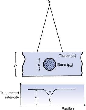
The fraction of the incident radiation transmitted through the thickness D−d of soft tissue is e−μ(T)(D−d). The total fraction can be found by adding the two fractions so that:
The difference between I2 and I1 is responsible for the contrast on the radiograph.
25.3.2 Scatter and the radiographic image
So far, the sections of this chapter have been oversimplified in that the emerging radiation beam is assumed to be composed only of transmitted primary beam. If only photoelectric absorption took place this would be true, but it is not true in the case of Compton scatter where only partial absorption of the photon energy occurs. This scattered radiation may escape from the patient and reach the image recording medium. Unfortunately, such scatter will form an image on the medium, but the image formed by the scatter forms an overall fog and so is not a useful image. Unless this scatter can be limited, serious image degradation can occur.
Scatter to the radiograph may be limited in two ways:
1. Limiting the amount of scatter formed.
2. Stopping any scatter formed from reaching the image recording medium.
Each of these will now be considered in turn.
25.3.2.1 Limiting scattered radiation formation
The amount of scatter formed in the patient depends on the number of atoms involved in scattering interactions. Thus, scatter formation is volume dependent, i.e. the greater the volume of patient irradiated, the greater the quantity of scatter formed. One of the major ways the operator can limit scatter formation is to reduce the volume of tissue irradiated. This can be done by collimation using a light-beam diaphragm or cones or, in some cases, by tissue displacement. Both these methods will not only produce an improvement in image quality but also reduce the radiation dose to the patient and others by limiting the scatter formation.
Most operators know from experience that the scattered radiation to the radiograph is increased as kVp is increased. This process is a somewhat complicated one. If the kVp is increased then photon energy is increased, and σ/ρ is proportional to 1/E. Thus, with higher-energy photons there are fewer scattering events within a given volume of tissue. With higher photon energy, the angle of scatter is smaller and consequently the scatter has a higher energy and is more likely to leave the body. We have more scatter leaving the patient and the scatter is in a more forward direction and so is more likely to hit the image receptor.
25.3.2.2 Stopping scatter from reaching the image receptor
Once formed, the most common way of stopping scatter from reaching the image receptor is to use a secondary radiation grid. Such a grid can remove about 90% of the scatter from the beam. A secondary radiation grid consists of strips of high-atomic-number material (e.g. lead) interspaced with strips of low-atomic-number material (e.g. carbon fibre). A section through such a grid is shown in Figure 25.3 where the lead strips are shaded. Primary radiation should hit the grid at right angles to its surface (or nearly right angles to it), so that it will easily pass between the lead strips (see ray 2 primary radiation (ray 1). may strike a lead strip and be absorbed. Because scatter (rays 3 and 4) are at an oblique angle to the primary beam these rays have an increased probability of striking a lead strip and being absorbed may strike a lead strip and be absorbed, if the angle is very small sees (ray 4) such scatter may’ miss’ the lead strip and strike the image receptor. Because scatter is at an oblique angle to the primary beam it has an increased probability of striking a lead strip and being absorbed. The fraction of the primary beam stopped is given by the ratio d/(D+d), since this is the fraction of the grid covered by lead; in practice this means the exposure must be increased when using a grid. Because scattered radiation is at an oblique angle to the primary beam, it has an increased probability of striking a lead strip and being absorbed. If the angle is very small, such scatter may be able to pass between the strips and reach the image receptor, but such rays do not contribute as much to image degradation as the more oblique rays.
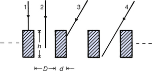
Figure 25.3 The principle of action of a secondary radiation grid. Scattered rays (3 and 4 in the diagram) are more likely to strike the lead and be absorbed by the lead than the primary rays (1 and 2 in the diagram).
Various factors of grid design may be chosen to optimize the performance of a secondary radiation grid for a particular application:

It can be appreciated from Figure 25.3 that increasing the height of the lead strips or reducing the space between them (i.e. increasing the grid ratio) will increase the efficiency of the grid in absorbing scattered radiation with a relatively small scatter angle
• The grid lattice or lattice density is a measure of the number of lines of absorber per centimetre. If we consider that the space between each strip is controlled by the grid ratio, then the number of lines per centimetre will affect the thickness of the individual lines. Grids with a high lattice density (i.e. 30–40 lines per centimetre) will have very fine lines and so do not degrade the image. If grid lattice density is low, the grid lines are visible which detract from image quality. A solution to this problem is to move the grid during the exposure so that the grid lines are blurred out. Such a device is known as a Potter–Bucky diaphragm or, more commonly, as a Bucky.
• As mentioned earlier, the grid will absorb some of the primary radiation and so it is necessary to increase the exposure when using a grid to compensate for this. The amount by which the exposure must be increased is known as the grid factor.
Note: This equation is only accurate if the kVp used for the exposure remains constant. A change of kVp will result in a change in the amount and type of scatter produced (see Insight, Sect. 25.3.2.1). It will also change the contrast range of the image (see Sect. 25.3.3). For most grids encountered in a diagnostic department, the grid factor will be between 2 and 6.
25.3.3 Effect of kVp on the X-ray image
The effect of a change of kVp on the spectrum of radiation produced by the X-ray tube has been discussed in Section 22.4 and, as can be seen from Figure 22.2, the average energy for a single-phase two-pulse generator is about one-third to one-half of the maximum photon energy. This means that if 90 kVp was applied across the X-ray tube, the maximum photon energy would be 90 keV, but the average photon energy would be approximately 40 keV. We can apply the various scattering and attenuation coefficients to a beam of radiation generated at 90 kVp that we would apply to a monoenergetic beam of photon energy of 40 keV. The effect of increasing kVp is to increase the average photon energy and reduce the linear attenuation coefficients of both bone and soft tissue. The radiation beam is more penetrating.
From Equation 25.2, it can be seen that increasing photon energy will reduce the amount of photoelectric absorption (τ) more than it will reduce Compton scattering (σ) because the photoelectric effect is proportional to I/E3. Because of less photoelectric absorption, there is less differentiation in absorption between bone and soft tissue – there is less contrast between the densities in the radiographic image. As already mentioned, an increase in kVp will also result in more scatter reaching the image receptor, further reducing contrast. Increasing kVp degrades image contrast in the ways mentioned above. There are practical advantages in using a high kVp. These are:
• It increases the intensity of the radiation beam, allowing a reduction in exposure time.
• It results in a higher percentage of the radiation beam being transmitted through the patient, again allowing a reduction in the exposure time.
• Because a higher percentage of the incident beam is transmitted through the patient, the absorbed radiation dose received by the patient is reduced.
The ‘best’ image is the one that most clearly demonstrates the structures we wish to see! There are some situations in which a low kVp is used to produce a high contrast between tissues of almost the same density (e.g. mammography) and others where we may wish to use a high kVp to demonstrate structures of very different radiopacity in the same image (e.g. high kV chest radiography).
25.4 The radioigraphic image pattern
The X-ray image pattern discussed so far in this chapter may be used to form an image on a number of different image receptors, for instance on a visual display unit (VDU), a photostimulable imaging plate (PSP) or even a film-intensifying screen combination, although the latter is very rarely used today.
When the image is displayed on a VDU, the light intensity is directly proportional to the radiation intensity, while a PSP has a similar linear response. This is not so when the radiation image is transferred to a photographic emulsion using intensifying screens. The intensifying screen produces light in proportion to the intensity of the X-ray image pattern. This light produces a latent image in the film. Processing then converts the invisible latent image into a permanent one. This blackening effect is not linear. An instrument called a densitometer, which is calibrated to measure optical density, can be used to assess the density or amount of blackening produced. Density is defined as log10(I0/It), where I0 is the intensity of the light on the processed film and It is the intensity of the light transmitted through it. Examination of a processed image will show that the darker the image, the less light transmitted through it and the higher the optical density. When plotting the density of the film at different exposures, it is usual to plot density against the logarithm of the relative exposure to accommodate the wide range of exposures to which the emulsion can respond. A graph of these densities can be produced; this is known as the characteristic curve of that emulsion.Figure 25.4 shows a typical characteristic curve.
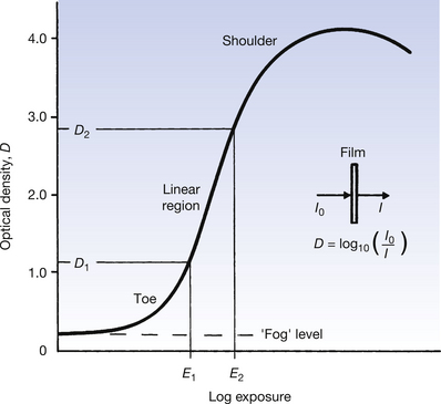
Figure 25.4 Response of a film screen combination obtained by plotting density against the log of the relative exposure.
Features of this graph will now be discussed (see Figure 25.4 page 188):
• Even when the relative exposure is zero, the emulsion will show some density. This is referred to as base plus fog. It results from the small amount of fog produced by the chemical activity of the developing process and any tint that may be present in the base material of the film. The density of this region is normally less than 0.2.
• There follows an initial horizontal portion where an increase in exposure produces no increase in density. This is often referred to as the threshold of the curve.
• The toe of the curve is the point at which the emulsion is becoming increasingly responsive to differences in exposure.
• There follows a region where an increase in exposure produces a linear increase in density. We aim to set X-ray exposure factors so that the exposure to the film falls in this part of the characteristic curve.
• The linear increase ‘flattens’ off at the shoulder. This usually occurs at densities between 3 and 4. We can only see contrasts between densities of just over 2 with the unaided eye; densities above this are seen as black. Industrial radiography makes use of this region.
In contrast, the PSP has a linear response over the entire exposure range, giving it a very high bit depth (see Ch. 34). Image processing software permits the selection of the range of the bit depth of the displayed image and also compensates for both over- and underexposure, although with gross underexposure, image pixelation is more noticeable.
25.5 Practical considerations in exposure selection
Where anatomical exposure selection in not available, the interrelationships between the various factors that affect image quality are complex and require considerable skill to master. There is a strong subjective element in selecting the ‘best’ image but no absolute rules can be laid down for exposure factors. The wide degree of variability in shape and size of the patients themselves, together with other practical difficulties (e.g. patients who are unable to keep still during the exposure), would provide so many exceptions that it is impossible to adhere to a strict set of rules. The operator’s experience is therefore critical in producing images of consistently high quality under all conditions. The following paragraphs should be considered with these general comments in mind.
In Chapter 22 we saw that, broadly speaking, the quality of the radiation in an X-ray beam depends on the kVp across the X-ray tube and the quantity of radiation produced on the mAs that flows through the X-ray tube during the exposure. If the kVp selected is too low, denser body structures (e.g. the bony skeleton) will not be penetrated by the X-ray beam resulting in excessive contrast and an increase in radiation dose to the patient. On the other hand, too high a kV reduces the contrast between structures and can produce significant amounts of scattered radiation. Unless this scatter is prevented from reaching the image receptor by the use of a secondary grid, image degradation can occur.
Image manipulation software can compensate for excessive density if too high an mAs is selected, but the operator may not be aware of their error and the patient will receive an excessive dose of radiation as a result. The exposure index shown on the monitor screen is an indicator of this. If the mAs selected is excessively low, image manipulation software can often produce an acceptable image, although pixelation may be present.
In this chapter, you should have learnt the following:
• How the X-ray beam is attenuated by bone and soft tissue (see Sect. 25.3.1).
• The effect of scattered radiation on the X-ray image and subsequently on the radiograph (Sect. 25.3.2).
• Methods of limiting the amount of scattered radiation formed (see Sect. 25.3.2.1).
• Methods of reducing the amount of scatter reaching the image receptor, including factors that affect the efficiency of a secondary radiation grid (see Sect. 25.3.2.2).
• The effect of a change of kVp on the X-ray image pattern (see Sect. 25.3.3).
• How the X-ray image pattern is changed into the radiographic image (see Sect. 25.4).
• What is meant by the characteristic curve of an emulsion (see Sect. 25.4).
• Practical considerations in the choice of exposure factors (see Sect. 25.5).
Further reading
Ball J.L., Moore A.D., Turner S. Ball and Moore’s Essential Physics for Radiographers, fourth ed. London: Blackwell Scientific, 2008. (Chapter 16)
Curry T.S.III, Dowdey J.E., Murry R.C.Jr. Christensen’s Physics of Diagnostic Radiography, fourth ed. London: Lee & Febiger, 1990. (Chapter 2)
Fauber T. Radiographic Imaging and Exposure, second ed. New York: Mosby, 2005. (Chapters 3 and 4)
Gunn C. Radiographic Imaging – A Practical Approach, third ed. Edinburgh: Churchill Livingstone, 2002. (Chapters 4, 5 and 8)
Webb S., editor, second ed. Bristol: Institute of Physics. 2000. (Chapter 2)