Advanced Imaging
The imaging modalities described in this chapter use equipment and techniques that are beyond the routine needs of most general dental practitioners. Each of these techniques makes a tomographic image, that is, a slice through tissue, rather than a simple projection image. The most versatile of these modalities are computed tomography (CT) and magnetic resonance imaging (MRI). Nuclear medicine and ultrasonography are used for more specialized applications. Film tomography, a mainstay imaging technique during the twentieth century, is being rapidly replaced by CT, MRI, and cone-beam imaging (Chapter 14). Each of these imaging modalities is used to aid in the diagnosis of conditions in the oral cavity; thus everyone involved in providing oral health care must have a basic understanding of their operating principles and clinical applications.
Computed Tomography
In 1972 Godfrey Hounsfield, an engineer, announced the invention of a revolutionary imaging technique that used image reconstruction mathematics developed by Alan Cormack in the 1950s and 1960s to produce cross-sectional images of the head. Currently this form of imaging is called computed tomography, abbreviated as CT. Hounsfield and Cormack shared the Nobel Prize in Physiology or Medicine in 1979 for their pioneering work.
COMPUTED TOMOGRAPHY SCANNERS
In its simplest form a CT scanner consists of an x-ray tube that emits a finely collimated, fan-shaped x-ray beam directed through a patient to a series of scintillation detectors or ionization chambers (Fig. 13-1, A). These detectors measure the number of photons that exit the patient. This information can be used to produce a cross-sectional image of the patient. In early versions of CT scanners, both the x-ray tube and detectors rotated synchronously about the patient. In more recent design the detectors form a continuous ring about the patient and the x-ray tube moves in a circle within the fixed detector ring (Fig. 13-1, B). Originally patients would lie on a stationary table while the x-ray source rotated one cycle around them. Then the table would move 1 to 5 mm for the next scan. CT scanners that used this type of “step and shoot” movement for image acquisition are called incremental scanners. The final image set consists of a series of contiguous or overlapping axial images, made at right angles to the long axis of the patient’s body. These two-dimensional slices are cross sections, typically 1 mm thick.
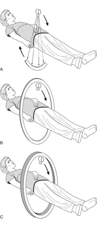
FIG. 13-1 Mechanical geometry of CT scanners.
A, In CT scanners the x-ray source emits a fan beam. In early CT scanners both the x-ray source and the detector array revolved around the patient. B, In current scanners the x-ray tube revolves around the patient and the remnant beam is detected by a fixed circular array. C, In contemporary CT multidetector scanners the detector array has 4 to 64 rows of detectors.
In 1989 CT scanners were introduced that acquire image data in a helical (sometimes inaccurately called spiral) fashion (Fig. 13-2). With helical scanners the gantry containing the x-ray tube and detectors continuously revolves around the patient, whereas the table on which the patient is lying continuously advances through the gantry. This results in the acquisition of a continuous helix of data as the x-ray beam moves down the patient. Helical CT is now the standard. In helical CT scanners, pitch refers to the amount of patient movement compared with the width of the image acquired. More precisely,
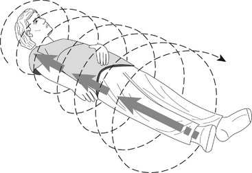
FIG. 13-2 Helical CT.
In helical scanners the patient is moves continuously through the gantry and the x-ray source moves continuously around the patient in a circle. The net effect is to describe a helical beam, and image, path through the patient.
A pitch of 1 means that the image width is equal to the amount of patient movement per slice. A pitch of 2 means that the patient moves twice as far as the detector is wide and only half the tissue is exposed. A pitch of 0.5 means that half the image is overlapped each slice. Overlapping reconstructions results in the highest spatial resolution but also the highest patient dose. Compared with incremental CT scanners, helical scanners provide improved multiplanar image reconstructions, reduced examination time, and a reduced radiation dose.
Multidetector helical CT (MDCT, multislice CT, or multirow CT) scanners were introduced in 1998. MDCT imaging has become widely used and has had a pronounced clinical impact. With this method, anywhere from four to 64 adjacent detector arrays are used in conjunction with helical CT (see Fig. 13-1, C). Additionally, the time for the x-ray tube to make a full cycle around the patient has been reduced to as little as 0.35 second. These developments allow images from multiple slices to be captured quickly and simultaneously, thus greatly reducing both exposure time and motion artifact from breathing, peristalsis, or heart contractions. This is important for patients who cannot hold their breath for long periods of time and for pediatric and trauma patients. The quality of axial, reformatted, and three-dimensional images is also greatly improved with MDCT compared with single-slice scanners. The meaning of pitch with MDCT varies with the individual manufacturer but often means that table travel per x-ray tube rotation divided by total active detector width. In general, the patient dose is higher with MDCT than with single-slice machines.
The most recent CT development is an electron beam CT. In this machine an electron gun generates an electron beam that is focused electrostatically on a fixed tungsten target circling halfway around the patient. The x rays that are generated expose the detector array circling the other half of the patient. Because there are no moving parts, an image may be acquired in less that 100 microseconds. This technique is primarily used for cardiac imaging to “stop” heart motion.
X-RAY TUBES
CT scanners use x-ray tubes with rotating anodes (see Fig. 1-10). These tubes have a high heat capacity, up to 8 million heat units]; (compare with dental tubes of 20 kilo heat units). They operate at 120 to 140 kilovolts peak (kVp) and 200 to 800 milliamperes. Focal spot sizes range from 0.5 to 2.0 mm. The high x-ray output minimizes exposure time and improves image quality by increasing the signal-to-noise ratio. The high kVp also provides a wide dynamic range by reducing bone absorption compared with soft tissue and extends tube life by reducing tube loading. The tubes operate continuously by using three-phase or high-frequency generators. The x-ray beam is collimated both before and after the patient. Prepatient collimation adjusts patient exposure. Postpatient collimation controls slice thickness. Slice thickness is typically between 1 and 3 mm. Thinner slices result in higher spatial resolution and contrast, less partial volume effect (see later), and higher patient dose.
DETECTORS
The x-ray beam exiting the patient is captured by an array of detectors. These detectors are usually gas filled or solid state. Gas-filled ion chamber detectors are usually made of high-pressure xenon. The ion chamber sends a signal proportional to the number of photons captured. Gas-filled ion chambers respond quickly but only capture about 50% of the photons in the beam. Solid-state detectors are used more commonly. These are usually made of cadmium tungstate, are optically coupled to a photodiode, and are as small as 0.625 mm across. These detectors are about 80% efficient. The signal from either type of detector is amplified, digitized, and sent to a computer for analysis.
IMAGE RECONSTRUCTION
The photons recorded by the detectors represent a composite of the absorption characteristics of all elements of the patient in the path of the x-ray beam. Computer algorithms use these photon counts to construct one, or more often, many digital cross-sectional images. The CT image is recorded and displayed as a matrix of individual blocks called voxels (volume elements) (Fig. 13-3). Each square of the image matrix is a pixel. Images are typically 512 × 512 or 1024 × 1024 pixels. Although the size of the pixel (about 0.6 mm or less) is determined partly by the computer program used to construct the image, the length of the voxel (about 1 to 20 mm) is determined by the width of the x-ray beam, which in turn is controlled by the prepatient and postpatient collimators. Next an interpolator algorithm is used to correct for the helical motion of the scanner and to construct planar cross sections from the helical information.
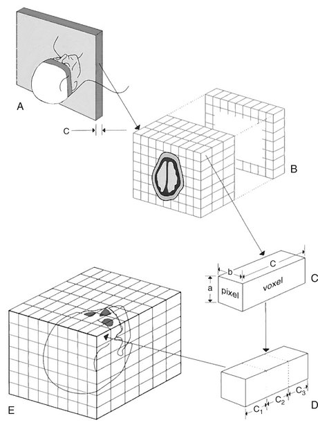
FIG. 13-3 CT Image Formation.
A, Data for a single-plane image are acquired from multiple projections made during the course of a 360-degree rotation around the patient. Slice thickness c is controlled by the width of the postpatient collimator. B, A single-plane image is constructed from absorption characteristics of the subject and displayed as differences in optical density, ranging from −1000 to +1000 HU. Several planes may be imaged from multiple contiguous scans. C, The image consists of a matrix of individual pixels representing the face of a volume called a voxel. Although dimensions a and b are determined partly by the computer program used to construct the image, dimension c is controlled by the collimator as in A. D, Cuboid voxels can be created from the original rectangular voxel by computer interpolation. This allows the formation of multiplanar and three-dimensional images (E).
The methods used to reconstruct images are complex. Initially an object with four compartments, as shown in Figure 13-4, should be pictured. The linear attenuation coefficients (densities) of each of the four cells can be computed by using four simultaneous equations to solve for four unknowns. This method becomes computationally impracticable when there are 5122 or 10242 cells. Instead, methods called filtered back-projection algorithms involving Fourier transformations are used for rapid image reconstruction. A modification of these methods, called the Feldkamp reconstruction, is used for MDCT and cone-beam reconstructions to account for the diverging x-ray beam. After reconstruction various image-processing filters are applied. Typically these are smoothing filters to minimize noise in low-contrast objects such as soft tissue and edge-sharpening filters to improve visualization of fine bony detail.
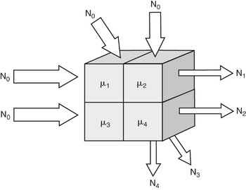
FIG. 13-4 Image reconstruction.
Assume four volumes with differing linear attenuation coefficients (μ). A beam entering the object with N0 photons is reduced in intensity by object. The intensity of the remnant beam is measured by the detector array. The value of each cell in the object can be determined by solving four (or more) independent simultaneous equations. Such a brute-force approach is computationally intensive and in practice much faster algorithms are used to reconstruct images.
COMPUTED TOMOGRAPHIC IMAGE
For image display, each pixel is assigned a CT number representing tissue density. This number is proportional to the degree to which the material within the voxel has attenuated the x-ray beam. CT numbers, also known as Hounsfield units (HU, named in honor of the inventor Sir Godfrey Hounsfield), range from −1000 to +1000, each corresponding to a different level of beam attenuation (Table 13-1). Some newer CT machines have a range of up to 4000 HU. Because the human eye can only detect about 40 shades of gray, it is useful to adjust the range and mean of CT numbers displayed on a monitor (Fig. 13-5). An image optimized for viewing bone, a “bone window,” may have a range (window width, or WW) of 700 units and mean of 500 (window level, or WL). Alternatively, an image optimized to view soft tissues may have a WW of 400 units and a WL of 40. In these images bone is light, soft tissue is gray, and air is black. By convention, these images are displayed as if the clinician is standing at the feet of the patient who is lying on his or her back. Thus the patient’s right side will appear on the left and anterior will appear at the top (Fig. 13-6, A).
TABLE 13-1
Typical Hounsfield Units for Air and Tissues
| TISSUE | HOUNSFIELD UNITS (CT NUMBERS) |
| Bone | +400 to +1000 |
| Soft tissue | +40 to +80 |
| Water | 0 |
| Fat | −60 to −100 |
| Lung | −400 to −600 |
| Air | −1000 |
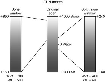
FIG. 13-5 Window Width and Level.
CT numbers, also called Hounsfield units (HU), are scaled on cortical bone (+1000), water (0), and air (−1000). Viewing bone or soft tissue is optimized by improving the contrast of the appropriate region of the original image. Window width (WW) is the range of CT numbers used, and window level (WL) is the mid portion of the range. Bone and soft tissue window views are used to enhance visualization of those tissues. In this example, a bone window may have a range of 700 and a mean of 500, whereas a soft tissue window may have a range of 400 and a mean of 40.
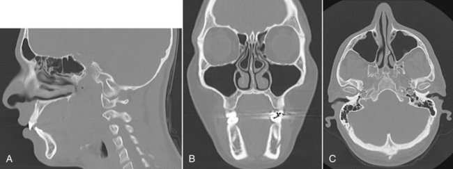
FIG. 13-6 Multiplanar Reconstruction Views Facilitate Interpretation of Complex Anatomy.
A, CT images demonstrating sagittal plane through lateral incisors and foramen lacerum. Note frontal, ethmoid, and sphenoid sinuses. B, Coronal view through ethmoid and maxillary sinuses and mental foramen in left mandible. C, Axial view through level of maxillary sinuses and mandibular condyles. Patient’s right side appear on the left side of the coronal and sagittal images as if the patient is lying on the back with the toes pointed toward the observer.
CT has several advantages over conventional film radiography and tomography. First, CT eliminates the superimposition of images of structures outside the area of interest. Second, because of the inherent high-contrast resolution of CT, differences between tissues that differ in physical density by less than 1% can be distinguished; conventional radiography requires a 10% difference in physical density to distinguish between tissues. Third, data from a single CT imaging procedure, consisting of either multiple contiguous or one helical scan, can be viewed as images in the axial, coronal, or sagittal planes, or in any arbitrary plane, depending on the diagnostic task. This is referred to as multiplanar reformatted imaging. Having the capability of viewing normal anatomy or pathologic processes simultaneously in three orthogonal planes greatly facilitates radiographic interpretation (Fig. 13-6).
Multiplanar images are two dimensional and require a certain degree of mental integration by the viewer for interpretation. This limitation has led to the development of computer programs that reformat data acquired from axial CT scans into three-dimensional images. The use of three-dimensional images has been boosted by the use of MDCT as a means of reviewing large amounts of information collected at each examination.
Three-dimensional reformatting requires that each original voxel, shaped as a rectangular solid, be dimensionally altered into multiple cuboidal voxels. This process, called interpolation, creates sets of evenly spaced cuboidal voxels (cuberilles) that occupy the same volume as the original voxel (see Fig. 13-4, D). The CT numbers of the cuberilles represent the average of the original voxel CT numbers surrounding each of the new voxels. Isotropic voxels as small as 0.24 mm can be achieved. Creation of these new cuboidal voxels allows the image to be reconstructed in any plane without loss of resolution by locating the position of each voxel in space relative to one another. In constructing the three-dimensional CT image, only cuberilles representing the surface of the object scanned are displayed on the monitor. The surface formed by these cuberilles is made to appear as if illuminated by a light source located behind the viewer (Fig. 13-7). In this manner the visible surface of each pixel is assigned a gray-level value, depending on its distance from and orientation to the light source. Thus pixels that face the light source or are closer to it appear brighter than those that are turned away from the source or are farther away. Once constructed, three-dimensional CT images may be further manipulated by rotation about any axis to display the structure imaged from any angle. Also, external surfaces of the image can be removed electronically to reveal concealed deeper anatomy.
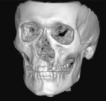
FIG. 13-7 Three-dimensional Surface Rendering.
Three-dimensional images can be reconstructed from the cuberilles, oriented in any arbitrary direction, and made to appear to have depth by highlighting structures near the front and shadowing structures near the back. Note cleft in left alveolar ridge of the left maxilla. Artifact from metallic restorations is also evident extending laterally from the occlusal plane. This image reconstructed from cone-beam data; see Chapter 14.
ARTIFACTS
Different types of artifacts may degrade CT images. Partial volume artifact occurs because a voxel has finite dimensions. When a voxel contains tissues of differing densities, for example, bone and soft tissue, the resulting CT number for that voxel is an intermediate value that does not represent either tissue. This may result in the resulting image as a blurring of the junction of the tissues or as a loss of part of a thin cortical layer of bone. Beam-hardening artifact results by the preferential absorption of lower energy photons in the heterogeneous x-ray beam. Because the distance through the center of the head is longer than along a path closer to the surface, there will be beam hardening seen as darkening in the middle of an axial slice. Software algorithms may minimize this artifact. Metal artifacts occur because of the near complete absorption of x-ray photons by metallic restorations. They appear as opaque streaks in the occlusal plane (see Fig. 13-6, B and C).
CONTRAST AGENTS
Contrast agents are substances used to improve visualization of structure. CT imaging frequently uses iodine, administered intravenously, to enhance soft tissue and vascular image detail. The iodine in the contrast medium has a large atomic number and thus effectively absorbs x rays (Fig. 13-8). Often malignant facial tumors are more vascularized than surrounding normal tissues; thus the presence of the iodine perfusing these tissues increases their radiographic density and makes their margins more detectable. Contrast medium also helps to visualize enlarged lymph nodes containing metastatic carcinoma. It should be remembered that contrast dye can be toxic to the kidneys in elderly individuals with kidney disease.
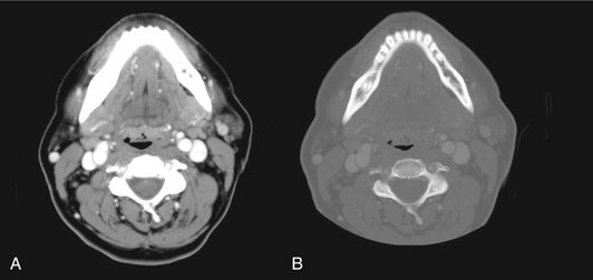
FIG. 13-8 Contrast agents.
Iodine may be administered intravenously to enhance blood vessels and structures with a rich vascular supply, including the periphery of some tumors. A, CT through mandible in soft tissue window and after administration of iodine. Note prominent great vessels lying just anterior and lateral to cervical vertebrae and muscles of floor of mouth and neck. B, Same axial slice displayed in bone window. Note presence of fine detail in mandible and cervical spine including cortical and cancellous bone and teeth, including their pulp chambers, but loss of soft tissue contrast.
APPLICATIONS
CT is useful for the diagnosis of and for determining the extent of a wide variety of infections, osteomyelitis, cysts, benign and malignant tumors, and trauma in the maxillofacial region. The ability of CT imaging to display fine bone detail makes it an ideal modality for lesions involving bone. Three-dimensional CT has been applied to trauma and craniofacial reconstructive surgery and has been used both for treatment of congenital and acquired deformities. The availability of data in a three-dimensional format also has allowed the construction of life-sized models that can be used for trial surgeries and the construction of surgical stents for guiding dental implant placement and for the creation of accurate implanted prostheses.
Magnetic Resonance Imaging
Paul Lauterbur described the first magnetic resonance image in 1973 and Peter Mansfield further developed use of the magnetic field and the mathematical analysis of the signals for image reconstruction. MRI was developed for clinical use around 1980. In 2003 Lauterbur and Mansfield were awarded the Nobel Prize in Physiology or Medicine.
To make a magnetic resonance image, the patient is first placed inside a large magnet. This magnetic field causes the nuclei of many atoms in the body, particularly hydrogen, to align with the magnetic field. The scanner then directs a radiofrequency (RF) pulse into the patient, causing some hydrogen nuclei to absorb energy (resonate). When the RF pulse is turned off, the stored energy is released from the body and detected as a signal in a coil in the scanner. This signal is used to construct the magnetic resonance image, in essence a map of the distribution of hydrogen.
MRI has the particular advantages of being noninvasive, using nonionizing radiation, and making high-quality images of soft tissue resolution in any imaging plane. Disadvantages of MRI include its high cost, long scan times, and the fact that various metals in the imaging field either will distort the image or may move in the strong magnetic field, injuring the patient.
PROTONS
Individual protons and neutrons (nucleons) in the nuclei of all atoms possess a spin, or angular momentum. In nuclei having equal numbers of protons and neutrons the spin of each nucleon cancels that of another, producing a net spin of zero. However, nuclei containing an unpaired proton or neutron have a net spin. Because spin is associated with an electrical charge, a magnetic field is generated in nuclei with unpaired nucleons, causing these nuclei to act as magnets with north and south poles (magnetic dipoles) and having a magnetic moment. The most common of these atoms, the magnetic resonance active nuclei, are hydrogen, carbon 13, nitrogen 15, oxygen 17, fluorine 19, sodium 23, and phosphorus 31. Hydrogen is by far the most abundant of these atoms in the body.
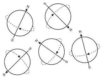
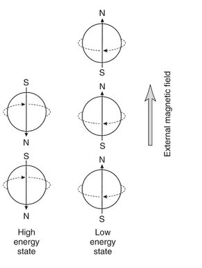
A hydrogen nucleus consists of a single unpaired proton and therefore acts as a magnetic dipole. Normally these magnetic dipoles are randomly oriented in space (Fig. 13-9). When an external magnetic field is applied, the hydrogen nuclear axes align in the direction of the magnetic field (Fig. 13-10). Two states are possible: spin-up, which parallels the external magnetic field, and spin-down, which is antiparallel with the field. Because more energy is required to align antiparallel with the magnetic field, those hydrogen nuclei are considered to be at a higher energy state than those aligned parallel with the field. Nuclei prefer to be in a lower energy state, and usually more are aligned parallel with the magnetic field. This results in a net magnetization vector in the direction of the magnetic field. Increasing the magnetic field strength increases the magnitude of the net magnetization vector.
PRECESSION
The magnetic moments of hydrogen nuclei in a magnetic field do not align exactly with the direction of the magnetic field. Instead, the orientations of the axes of spinning protons actually oscillate with a slight tilt from a position absolutely parallel with the flux of the external magnet (Fig. 13-11). This tilting of the spin axis, called precession, is similar to that of a spinning toy top, which rotates around an upright position as it slows down. Similarly, the presence of the magnetic field causes the axis of the spinning proton to wobble (or precess) around the lines of the applied magnetic field (Fig. 13-12). The rate or frequency of precession is called the precessional, resonance, or Larmor frequency. The precessional frequency depends on the species of nucleus (hydrogen nucleus or other) and is proportional to the strength of the external magnetic field. The magnetic field in a magnetic resonance scanner is provided by an external permanent magnet. Magnetic resonance field strengths range from 0.1 to 4 Tesla (T) with 1.5 T being the most common. (1.5 T is about 30,000 times the strength earth’s magnetic field.) The Larmor precession frequency of hydrogen is 63.86 megahertz in a magnetic field of 1.5 T. Other magnetic resonance active nuclei precess at different frequencies in the same magnetic field.
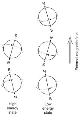
FIG. 13-11 Hydrogen Nuclei in an External Magnetic Field.
The magnetic dipoles are not aligned exactly with the external magnetic field. Instead, the axes of spinning protons actually oscillate or wobble with a slight tilt from being absolutely parallel with the flux of the external magnet.
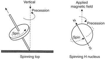
FIG. 13-12 Precession.
Much as a top rotates around a vertical axis when spinning, a spinning hydrogen nucleus rotates around the direction of the external magnetic field. This movement is called precession and the rate or frequency of precession is called the precessional, resonance, or Larmor frequency. The Larmor frequency depends on the strength of the external magnetic field and is specific for the nuclear species.
RESONANCE
Nuclei can be made to undergo transition from one energy state to another by absorbing or releasing energy. Energy required for transition from the lower to the higher energy level can be supplied by electromagnetic energy in the RF portion of the electromagnetic spectrum. In an MRI scanner the RF broadcast from an antenna coil is directed to tissue with protons (hydrogen nuclei) aligned in the Z axis (long axis of a patient) by the external static magnetic field (Fig. 13-13). When the frequency of the RF pulse matches the Larmor frequency of the protons in the tissue, the protons resonate and absorb the RF energy. This causes some of the low-energy nuclei (parallel) to gain energy to convert to the high-energy (antiparallel) state. As a consequence, the longitudinal magnetic vector is reduced. The longer the RF pulse is applied, the less the longitudinal magnetic vector. The RF pulse also causes the protons to precess in phase with each other, resulting in a net tissue magnetization vector in the transverse plane (XY plane) perpendicular to longitudinal alignment (Z axis) (Fig. 13-14). If the RF pulse is of sufficient intensity and duration, the longitudinal magnetic vector is reduced to zero. An RF pulse that accomplished this is called a 90-degree RF pulse or having a flip angle of 90 degrees. At this time the net magnetic vector in the transverse plane is maximized because the magnetic moments of all nuclei are in phase.
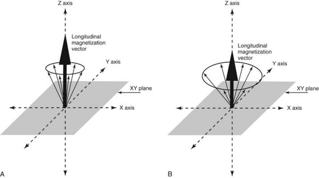
FIG. 13-13 Longitudinal Magnetic Vector.
When hydrogen nuclei are in an external magnetic field, two energy states result: spin-up, which is parallel to the direction of the field, and spin-down, which is antiparallel to the direction of the field. A, The combined effect of these two energy states is a weak net magnetic moment, or magnetization vector parallel with the applied magnetic field. B, When the frequency of the RF pulse matches the Larmor frequency of the protons absorb the RF energy causing some low-energy nuclei to convert to the high-energy state, thereby reducing the net longitudinal magnetic vector, vertical black arrow in Z axis.
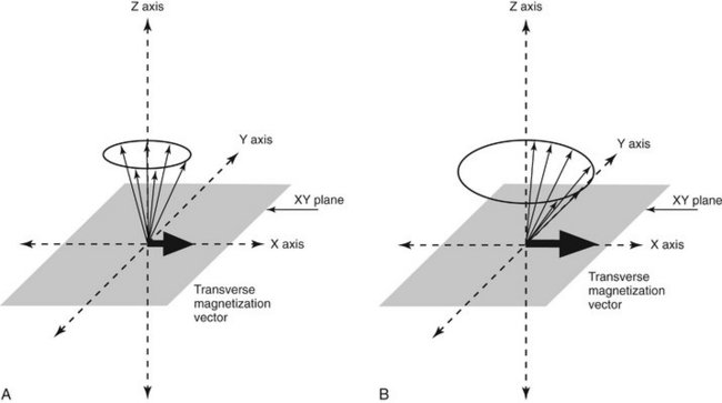
FIG. 13-14 Transverse Magnetic Vector.
A, The RF pulse also causes the protons to precess in phase with each other, resulting in a net tissue magnetization vector in the transverse plane (XY plane). B, Increasing the intensity and duration RF of the pulse increases the transverse magnetization vector because the nuclei are more nearly in phase, horizontal black arrow in X axis.
MAGNETIC RESONANCE SIGNAL
The precession of the net magnetic vector, that is, the precession of the magnetic moments of the hydrogen nuclei in phase in the transverse plane, induces a current flow in a receiver coil (Fig. 13-15), the MR signal. The frequency of this alternating current signal matches the frequency of the RF pulse and the Larmor precessional frequency of hydrogen nuclei. The magnitude of this signal is proportional to the overall concentration of hydrogen nuclei (proton density) in the tissue. This strength of the signal also depends on the degree to which hydrogen is bound within a molecule. Tightly bound hydrogen atoms, such as those present in bone, do not align themselves with the external magnetic field and produce only a weak signal. Loosely bound or mobile hydrogen atoms such as those in soft tissues and liquids react to the RF pulse and thus produce a detectable signal at the end of the RF pulse. The concentration of loosely bound hydrogen nuclei available to create the signal is referred to as the proton density or spin density of the tissue in question. The higher the concentration of these nuclei of loosely bound hydrogen atoms, the stronger the net transverse magnetization, the more intense the recovered signal, and the brighter the corresponding part of the magnetic resonance image.
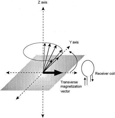
FIG. 13-15 Receiver coil.
The precession of the net transverse magnetic vector in the XY plane induces a current flow in a receiver coil, the magnetic resonance signal. The frequency of this induced alternating current signal matches the frequency of the RF pulse and the Larmor precessional frequency of hydrogen nuclei.
When the RF pulse is turned off, the nuclei begin to return to their original lower-energy spin state, a condition called relaxation. As they give up the energy absorbed by the RF pulse, some of the high-energy nuclei return to the low-energy state and the net longitudinal magnetic vector returns to its original state. Additionally, and independently, the individual magnetic moments of the protons begin to interact with each other and dephase. This results in reduction of the magnetization in the transverse plane, a condition called decay. As a result of the loss of transverse magnetization and the dephasing of the hydrogen nuclei, there is a loss of intensity of the magnetic resonance signal. The reduced voltage induced in the receiving coil is called the free induction decay (FID) signal. In sum, the FID of the MR signal results from the loss of the transverse net magnetization vector. This results from return of the net magnetization vector to the longitudinal plane and dephasing of the hydrogen nuclei.
T1 AND T2 RELAXATION
Relaxation at the end of the RF pulse results in recovery of the longitudinal magnetization. This is accomplished by a transfer of energy from individual hydrogen nuclei (spin) to the surrounding molecules (lattice). This is an exponential process and the time required for 63% of the net magnetization to return to equilibrium (the time constant) by this transfer of energy is called the T1 relaxation time or spin-lattice relaxation time. The T1 relaxation time varies with different tissues and reflects the ability of their nuclei to transfer their excess energy to surrounding molecules (Table 13-2).
TABLE 13-2
T1 and T2 Relaxation Times in a Main Field of 1.5 Tesla
| TISSUE TYPE | T1 TIME (MS) | T2 TIME (MS) |
| Fat | 240-250 | 60-80 |
| Bone marrow | 550 | 50 |
| White matter of cerebrum | 780 | 90 |
| Gray matter of cerebrum | 920 | 100 |
| Muscle | 860-900 | 50 |
| CSF (similar to water) | 2200-2400 | 500-1400 |
CSF, Cerebrospinal fluid.
Additionally, and the end of the RF pulse, the magnetic moments of adjacent hydrogen nuclei begin to interfere with one another, causing the nuclei to dephase with a resultant loss of transverse magnetization. The time constant that describes the exponential rate of loss of transverse magnetization is called the T2 relaxation time or the spin-spin relaxation time. As the transverse magnetization rapidly decays to zero, so does the amplitude and duration of the detected radio signal. T2 relaxation occurs more rapidly than T1 relaxation. Note that both T1 and T2 times are features of the tissues being examined.
RADIOFREQUENCY PULSES SEQUENCES (AND IMAGE CONTRAST)
The components of the RF pulse sequence are set by the operator and determine the appearance of the resultant image. The most basic features of a pulse sequence are the repetition time (TR) and echo time (TE). The TR time is the duration between repeat RF pulses (Fig. 13-16). The time between pulse repetitions determines the amount of T1 relaxation that has occurred at the time the signal is collected. The TE time is the time after application of the RF pulse when the magnetic resonance signal is read. It controls the amount of T2 relaxation that has occurred when the signal is collected. There are many sequences that can be used to emphasize various features of the tissues being examined.
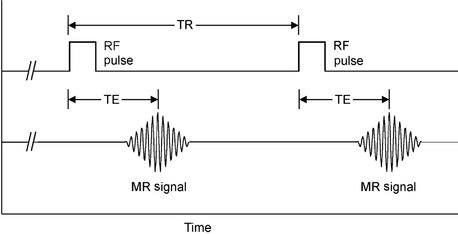
FIG. 13-16 RF Pulses Sequences.
The most basic features of a pulse sequence are the TR, the duration between repeat RF pulses, and the TE, the time after application of the RF pulse when the magnetic resonance signal is read. TR determines amount of T1 relaxation that has occurred at the time the signal is collected, whereas TE controls the amount of T2 relaxation that has occurred when the signal is collected.
TISSUE CONTRAST
Image contrast between tissues is governed by intrinsic features of the tissues, including proton density, T1 and T2 times of the issues being imaged, and how the TR and TE times are adjusted to emphasize these features. For instance, a tissue that has a high proton density and strong transverse magnetization vector (protons precessing in phase) at TE will produce a strong magnetic resonance signal that will appear bright on a magnetic resonance image. Conversely, a tissue with a low proton density or low transverse magnetization vector at TE produces a weak signal and appears dark on a magnetic resonance image.
T1-Weighted Image
A T1-weighted image emphasizes differences in T1 values of tissues (Fig. 13-17, A). This is accomplished by use of short TR times, typically 300 to 700 ms, and short TE times (20 ms). In such images tissues with fast T1 times, such as fat, will appear bright, whereas those with long T1 times, such as cerebrospinal fluid (CSF) (water), will appear dark. T1-weighted images are more commonly used to demonstrate anatomy.
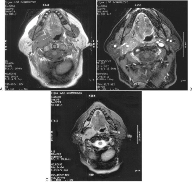
FIG. 13-17 MRI images.
MRI examination performed to evaluate neck mass in a patient with known diagnosis of multiple myeloma. A, Axial T1 precontrast (no fat saturation) image through mandible. Note abnormally dark marrow in posterior right mandible (arrow, compare with left side) and mass in right carotid space (other arrow). B, Axial T1 postcontrast image with fat saturation. Note abnormal enhancement of both marrow in right mandible and of the mass in the right carotid space. C, Axial T2 with fat saturation demonstrating abnormally bright signal in both marrow in right mandible and of the mass in the right carotid space. (Courtesy Dr. Thomas Underhill, Radiology Associates, Richmond, Va.)
T2-Weighted Image
A T2-weighted image emphasizes differences in T2 values of tissues (Fig. 13-17, B). This is accomplished by use of long TR times (2000 ms) and long TE times, typically 60 ms or more. In such images tissues with long T2 times, such as CSF for temporomandibular (TMJ) joint fluid, will appear bright, whereas tissues with short T2 times, such as fat, will appear dark. Images with T2 weighting are most commonly used for identifying inflammatory or other pathologic changes.
There are many pulse sequences involving varying the strength and timing of the RF pulses that emphasize or suppress various tissues in the resultant images. Techniques such as spin echo and gradient echo allow images to be captured rapidly. Other techniques allow the signal from fat, or water, to be enhanced or suppressed. A technique called “fat saturation” nulls the signal from fat.
Contrast Agents
Contrast agents, most commonly gadolinium, may be administered intravenously to improve tissue contrast (Fig. 13-17, C). Gadolinium is not imaged itself, but rather it shortens the T1 relaxation times of enhancing tissues, making them appear brighter. It is useful for enhancing some tumors by allowing them to be better differentiated from surrounding normal tissue. For imaging the head and neck, it is common practice to obtain T1, T1 postgadolinium administration and with fat saturation, and T2 with fat saturation images. It should be noted that just recently there is evidence that gadolinium-based contrast media could be a cause of a debilitating disease called nephrogenic systemic fibrosis in some patients with renal dysfunction. The implications of this finding are under active study.
SCANNER GRADIENTS
To generate an image, a magnetic resonance signal must be collected from a discrete slice of tissue in the patient. This is accomplished by using three gradient coils within the bore of the imaging magnet oriented in the X (left to right), Y (anterior to posterior), and Z (head to toe) planes. The intensity of the magnetic field surrounding a patient may be modified with these gradient coils. When one of coils is turned on, it creates a gradient in the intensity of the magnetic field. Thus in a 1.5 T scanner, when the Z-axis gradient is turned on, the strength of the magnetic field at the head might be 1.4 T and that at the toe 1.6 T. When this gradient field is applied, the precessional frequency of hydrogen nuclei will vary linearly along the magnetic gradient. Accordingly, when an RF pulse is applied, only those nuclei precessing at the same frequency as the applied signal will resonate. This allows selecting the desired slice of tissue along the patient’s long axis (Z gradient). The slope of the gradient applied and the bandwidth of the RF pulse determine the thickness of this slice. The location of the signal within the X and Y (transverse) planes of the selected longitudinal plane is derived by switching off the Z-gradient coil followed by rapidly turning on the X- and then the Y-gradient coils (phase encoding and frequency encoding, respectively). This sequence alters the phase and precessional frequencies of the nuclei in the selected slice. The resulting magnetic resonance signal from the patient is read out while the frequency-encoding gradient is applied. The signal from the patient contains many frequencies that is decomposed by the fast Fourier transform into amplitude and frequency. This information, which reflects the number of hydrogen nuclei and their T1 and T2 properties at each X and Y location in the selected longitudinal plane, is reconstructed into magnetic resonance images.
MAGNETIC RESONANCE IMAGES
MRI has several advantages over other diagnostic imaging procedures. First, it offers the best contrast resolution of soft tissues. Although x-ray attenuation coefficients of soft tissues may vary by no more than 1%, T1 and T2 relaxation times may vary by up to 40%. Second, no ionizing radiation is involved with MRI. Third, because the region of the body imaged in MRI is controlled with the gradient coils, direct multiplanar imaging is possible without reorienting the patient. Disadvantages of MRI include relatively long imaging times and the potential hazard imposed by the presence of ferromagnetic metals in the vicinity of the imaging magnet. This latter disadvantage excludes from MRI any patient with implanted metallic foreign objects or medical devices that consist of or contain ferromagnetic metals (e.g., cardiac pacemakers, some cerebral aneurysm clips or ferrous foreign bodies in the eye). The strong magnetic fields may move these objects and harm patients. Metals used in dentistry for restorations or orthodontics will not move but may distort the image in their vicinity. Titanium implants cause only minor image degradation. Finally, some patients have claustrophobia when positioned in an MRI machine.
APPLICATIONS
Because of its excellent soft tissue contrast resolution, MRI is useful in evaluating soft tissue conditions, for instance, the position and integrity of the disk in the TMJ (Fig. 13-18); for soft tissue disease especially neoplasia involving the soft tissues, such as tongue, cheek, salivary glands, and neck; determining malignant involvement of lymph nodes; and determining perineural invasion by malignant neoplasia. Similar to CT imaging, a contrast agent such as gadolinium can be added to enhance the image resolution of neoplasia (Fig 13-19). Also, it is customary to remove the high signal of surrounding fat tissue (fat suppression) to enhance the appearance of the neoplasm. A typical protocol would include T1, T1 postgadolinium (with fat suppression), and T2 (with fat suppression) images.
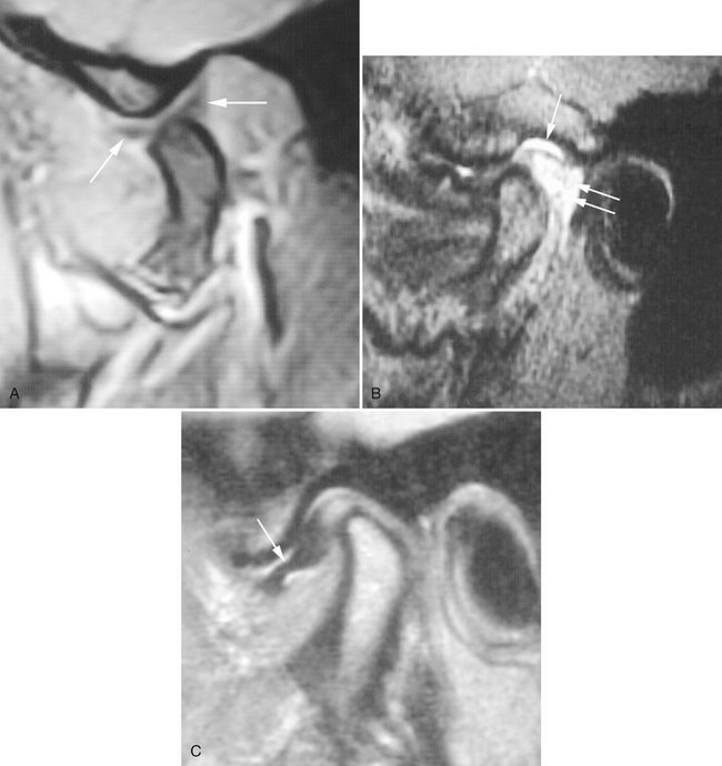
FIG. 13-18 Magnetic resonance of TMJ.
A, T1-weighted magnetic resonance image of the TMJ. In this image the jaw is partly open, as indicated by the location of the condyle relative to the articular eminence. The articular disk, which has a “bow tie” appearance (arrows), is in a normal position relative to the translating condyle. B, T2-weighted magnetic resonance image of the TMJ. This image illustrates both inflammatory effusion into the superior joint space (arrow) and hyperemia caused by increased vasculature in the retrodiskal tissues (double arrows). C, Proton or spin density magnetic resonance image of the TMJ. In this image the disk is anteriorly displaced (arrow), with the posterior band in the 9 o’clock position relative to the condylar head. (B and C, Courtesy Richard Harper, DDS, Dallas, Tex.)
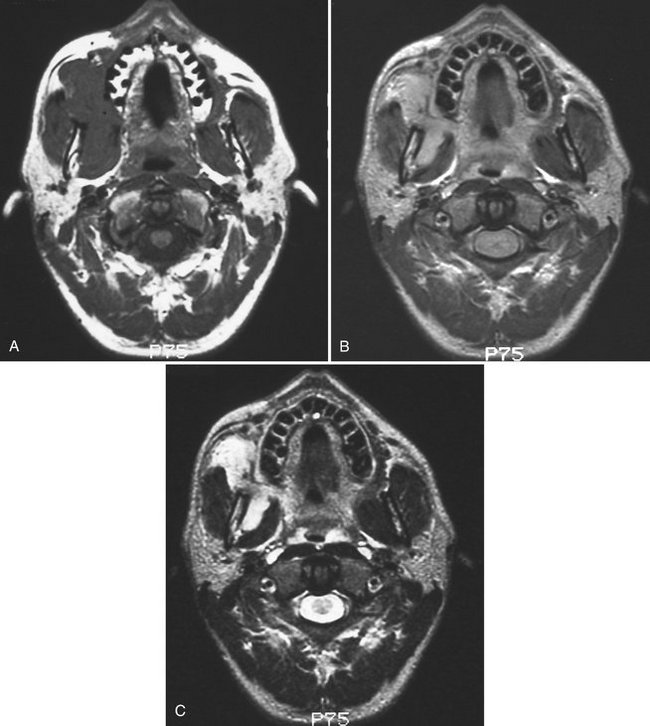
FIG. 13-19 Gadolinium Enhancement of Magnetic Resonance Image.
A, Axial T1 magnetic resonance image of a rabdomyosarcoma involving the soft tissues of the right face. The tumor cannot be distinguished from the adjacent masseter and pterygoid muscles because both have the same tissue signal. B, Axial T1 postgadolinium magnetic resonance image of same case. Note that the tumor now has a brighter signal (lighter) than the adjacent muscles because of its greater vascularity, enhanced by the gadolinium. C, Axial T2 magnetic resonance image of same case. Note that the tumor has a brighter signal than adjacent muscles because of greater fluid content of the tumor.
Nuclear Medicine
Film radiography, CT, MRI, and diagnostic ultrasonography are morphologic imaging techniques in that each requires a macroscopic anatomic change for information to be recorded by an image receptor. However, in some human diseases abnormal biochemical processes occur without anatomic change. Radionuclide imaging (a form of functional imaging) provides a means of assessing such physiologic change. Nuclear medicine examinations are commonly used for assign function of the brain, thyroids, heart, lungs, and gastrointestinal system as well as for diagnosis and follow-up of metastatic disease, bone tumors, and infection (Fig. 13-20).
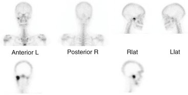
FIG. 13-20 Radionuclide image.
The increased uptake of 99mTc-MDP in the region of the right TMJ. The top row images were captured with a γ-scintillation camera. The lower two tomographic images were captured with SPECT.
Radionuclide imaging uses radioactive atoms or molecules that emit gamma rays. These atoms behave in an organism in a manner comparable to their stable counterparts because they are chemically indistinguishable. Radionuclides allow measurement of tissue function in vivo and provide an early marker of disease through measurement of biochemical change. After the radionuclides are administered, they distribute in the body according to their chemical properties. The γ-scintillation camera detects gamma rays and forms planar images showing the locations of the radionuclides in the body. Single photon emission computed tomography (SPECT) and positron emission tomography (PET) imaging are advanced nuclear medicine techniques that form tomographic views. Recently molecular imaging of individual gene expression is being accomplished in the laboratory.
RADIONUCLIDES
The ideal radionuclide has a short half-life, emits γ rays but no charged particles, and is capable of binding to a variety of pharmaceuticals. Although many γ-emitting isotopes are used in radionuclide imaging, including iodine (131I), gallium (67Ga), and selenium (74Se), the most commonly used is technetium 99m (99mTc). Technetium 99m has a half-life of 6 hours and emits primarily 140 kiloelectron volt (keV) photons. As technetium pertechnetate, 99mTc mimics iodine distribution when injected intravenously and is concentrated by the salivary and thyroid glands and gastric mucosa. When it is attached to various carrier molecules, it can be used to examine virtually every organ of the body.
To image bone, 99mTc is typically bound to methylene diphosphonate (MDP) and a dose of 20 to 30 mCi (740 to 1110 mega-Becquerels [MBq]) is injected intravenously. Immediately after injection the tracer distributes intravascularly. Images made during this flow phase, the first 60 to 90 seconds, are called radionuclide angiography. In the second, or blood pool phase, the tracer quickly moves into the extracellular space. The third, or bone scintigraphy phase, is made 2 to 3 hours after injection. The MDP deposition in the skeleton depends both on osteoclastic activity and blood flow (Fig. 13-20). Images made 2 to 3 hours after injection show most of the tracer activity in the skeleton, kidneys, and bladder. Most metastatic tumors in bone induce formation of new bone and thus may be detected on such an examination.
Radionuclide-labeled tracers are used in quantities well below amounts that are lethal to cells. However, although radionuclide imaging is considered noninvasive, the radiation dose the patient receives as a result of intravenous injection of radionuclide-labeled tracers should be considered. Injection of 740 MBq of 99mTc pertechnetate delivers a whole-body radiation dose of 2 milliGrays (mGy). This quantity is less than the average annual effective dose resulting from natural radiation (see Chapter 3).
γ-SCINTILLATION CAMERA
γ-Scintillation cameras (also called Anger cameras) are the most common means of forming an image (Fig. 13-21). These cameras capture photons and convert them to light and then to a voltage signal. This signal is reconstructed to a planar image that shows the distribution of the radionuclide in the patient. The first part of the gamma camera is a collimator. It absorbs γ rays that do not travel parallel to the plates, thus improving image resolution. The γ rays that pass through the collimator then strike a scintillation crystal. This crystal, often made of sodium iodide with trace amounts of thallium, fluoresces when it absorbs γ rays. These flashes of light are detected by an array of photomultiplier tubes coupled to the crystal with light pipes. The photomultiplier tubes capture the flash and amplify the signal. The size of the signal is proportional to the energy of the absorbed photon. The signals from the photomultiplier tubes go through an analog to digital converter and then to a pulse height analyzer. This device detects the intensity of the signal, and thus the energy of the incident absorbed photons, and only uses those from the radionuclide when forming the final image. Many of the γ rays released from the radionuclide in the patient undergo Compton absorption at some distant site and result in a new scattered photon. If these scattered, lower-energy photons pass through the collimator of the gamma camera, they may degrade image resolution. However, these scattered photons are detected by the pulse height analyzer and are rejected so that they do not contribute to the image. Gamma cameras have a spatial resolution of up 3 to 5 mm. Use of a scintillation crystal for acquisition of data for image formation has led to the labeling of this technique as scintigraphy.
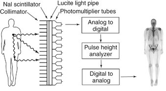
FIG. 13-21 Gamma Scintillation camera.
The principal components of a gamma scintillation camera are a collimator to limit γ rays to those perpendicular to the surface of the camera, a scintillator to absorb the γ rays and emit a flash of visible light, photomultiplier tubes to count the flashes of light and measure their energy, a pulse height analyzer to select only those flashes from the administered radionuclide, and a monitor to display the resultant image. The most superior γ ray will pass through the collimator and contribute to the image and the collimator will block the second γ ray. The photon resulting from Compton scattering in the leg will be rejected by the pulse height analyzer and not contribute to the image. Image of patient is anterior view of patient after intravenous injection of 99mTc-MDP.
SINGLE PHOTON EMISSION COMPUTED TOMOGRAPHY
SPECT is a method of acquiring tomographic slices through a patient. Most gamma cameras have SPECT capability. In this technique either a single or multiple gamma camera is rotated 360 degrees about the patient. Image acquisition takes about 30 to 45 minutes. The acquired data are processed by filtered back projection and, more recently, iterative reconstruction algorithms, to form a number of contiguous axial slices, similar to CT by x ray. These data can then be used to construct multiplanar images of the study area (see Fig. 13-20). Tomography enhances contrast and removes superimposed activity. Recently SPECT images have been fused with CT images to improve identifying of the location of the radionuclide.
APPLICATIONS
The maxillofacial region most common use of nuclear medicine is to investigate abnormal metabolic bone activity, for instance, in assessing growth activity in cases of condylar hyperplasia and presence of metastatic lesions. Traditionally a combination of 99mTc MDP and gallium citrate was used to diagnose osteomyelitis, but CT imaging is now used more frequently.
POSITRON EMISSION TOMOGRAPHY
PET is a more advanced imaging modality in nuclear medicine. PET, which is reported to have a sensitivity nearly 100 times that of a gamma camera, relies on positron-emitting radionuclides generated in a cyclotron. The utility of PET is based not only on its sensitivity but also on the fact that the most commonly used radionuclides (11C, 13N, 15O, 18F) are isotopes of elements that occur naturally in organic molecules. Although fluorine does not technically fit into this category, it is a chemical substitute for hydrogen. These radionuclides are used as is, or more commonly, incorporated into a radiopharmaceutical such as glucose or amino acids by use of a medical cyclotron. After the radiopharmaceutical is injected into the patient, the isotope distributes within the body’s tissue according to the carrier molecule and emits a positron. This positron then interacts with a free electron and mutual annihilation occurs, resulting in the production of two 551-keV photons emitted at 180 degrees to each other. The PET scanner consists of a ring of many detectors in a circle around the patient (Fig. 13-22). The detector crystals are often made of bismuth germinate. Electronically coupled opposing detectors simultaneously identify the pair of γ photons using coincidence detection circuits that measure events within 10 to 20 nanoseconds. The annihilation event is thus known to have occurred along the line joining the two detectors. Raw PET scan data consist of a number of these coincidence lines, which are reorganized into projections that identify where isotope is concentrated within the patient. The spatial resolution of a PET scanner is about 5 mm. PET is useful in skeletal imaging for assessing primary bone tumors, locating metastases in bone, and detecting osteomyelitis. For instance, 18F-fluoro-2-deoxyglucose (18F-FDG) is a radiopharmaceutical commonly used for studying glucose use in the brain and heart and to look for cancer metastases (Fig. 13-23). PET images are often fused with CT scans to facilitate anatomic localization of radionuclide. The PET/CT combination has been shown to be quite helpful in staging and treatment planning of squamous cell carcinoma in the head and neck.
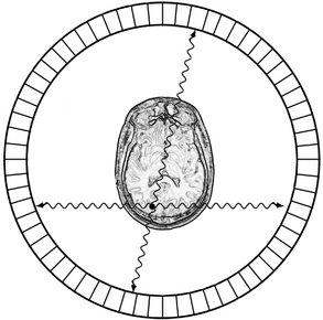
FIG. 13-22 PET scanner.
A PET scanner consists of a ring of detectors that measure pairs of 511 keV γ rays traveling in opposite directions from positron annihilation. Each pair is recorded simultaneously; thus the location of the radionuclide can be determined as the intersection of the pairs of detectors recording simultaneous events. The location of the common source of the radionuclide is thus readily determined as the intersection of the flight paths of the γ rays.
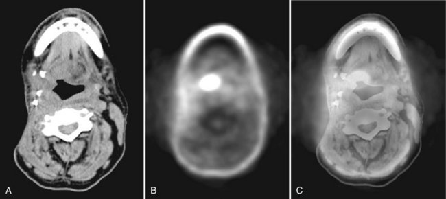
FIG. 13-23 PET Scan and Fused PET-CT.
This patient has a known recurrent carcinoma at the base of the tongue. A, Soft-tissue algorithm CT at level of inferior border of mandible. The four metallic objects on the patient’s right side posterior to the mandible represent vascular clips from prior surgery. B, FDG PET scan showing oval-shaped region of high metabolic activity of tumor at the right tongue base. The FDG activity in the anterior mandible is related to low level metabolic activity in the vicinity of a reconstruction plate. C, Fused images A and B demonstrating the region of high metabolic activity superimposed on the CT anatomy. Images acquired on combined PET-CT scanner. (Courtesy Dr. Todd W. Stultz, Cleveland Clinic, Ohio.)
Ultrasonography
Sonography is a technique based on sound waves that acquires images in real time and without the use of ionizing radiation. The phenomenon perceived as sound is the result of periodic changes in the pressure of air against the eardrum. The periodicity of these changes lies anywhere between 1500 and 20,000 Hz. By definition, ultrasound has a periodicity greater than 20 kHz, greater than the audible range. Diagnostic ultrasonography (sonography), the clinical application of ultrasound, uses vibratory frequencies in the range of 1 to 20 MHz.
Scanners used for sonography generate electrical impulses that are converted into ultra-high-frequency sound waves by a transducer, a device that can convert one form of energy into another—in this case, electrical energy into sonic energy. The most important component of the transducer is a thin piezoelectric crystal or material made up of a great number of dipoles arranged in a geometric pattern. A dipole may be thought of as a distorted molecule that appears to have a positive charge on one end and a negative charge on the other. Currently, the most widely used piezoelectric material is lead zirconate titanate. The electrical impulse generated by the scanner causes the dipoles in the crystal to realign themselves with the electrical field and thus suddenly change the crystal’s thickness. This abrupt change begins a series of vibrations that produce the sound waves that are transmitted into the tissues being examined.
The transducer emitting ultrasound is held against the body part being examined. The ultrasonic beam passes through or interacts with tissues of different acoustic impedance. Sonic waves that reflect (echo) toward the transducer cause a change in the thickness of the piezoelectric crystal, which in turn produces an electrical signal that is amplified, processed, and ultimately displayed as an image on a monitor. Typically the transducer serves as both a transmitter and a receiver. Current techniques permit echoes to be processed at a sufficiently rapid rate to allow perception of motion; this is referred to as real-time imaging.
The ultrasound signal transmitted into a patient is attenuated by a combination of absorption, reflection, refraction, and diffusion. The higher the frequency of the sound waves, the higher the image resolution but the less the penetration of the sound through soft tissue. The fraction of the beam that is reflected to the transducer depends on the acoustic impedance of the tissue, which is a product of its density (and thus the velocity of sound through it) and the beam’s angle of incidence. Because of its acoustic impedance, a tissue has a characteristic internal echo pattern. Consequently, not only can changes in echo patterns distinguish between different tissues and boundaries, but they also can be correlated with pathologic changes within a tissue. Tissues that do not produce signals, such as fluid-filled cysts, are said to be anechoic and appear black. Tissues that produce a weak signal are hypoechoic, whereas tissues that produce intense signals such as ligaments, skin, or needles or catheters are hyperechoic and appear bright. Interpretation of sonograms thus relies on knowledge of both the physical properties of ultrasound and the anatomy of the tissues being scanned.
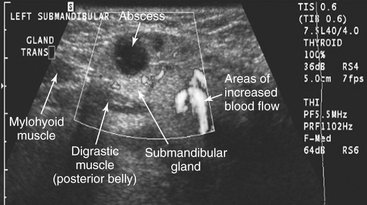
Ultrasonography is used in the head and neck region for evaluating for neoplasms in the thyroid, parathyroid or salivary glands or lymph nodes, for stones in salivary glands or ducts, Sjögren’s syndrome, and the vessels of the neck, including the carotid for atherosclerotic plaques (Figs. 13-24 and 13-25). Ultrasonography is also used to guide fine-needle aspiration in the neck. Recent advances include three-dimensional imaging to allow multiplanar reformatting, surface renderings (for example of a fetal face), and color Doppler sonography for evaluation blood flow.
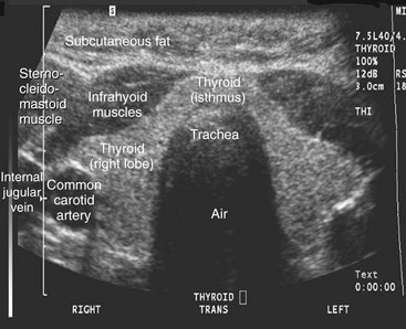
FIG. 13-24 Ultrasound examination (transverse section) of a healthy thyroid gland. This image shows glandular, muscular, adipose, and vascular tissues because of the different acoustic impedance of these tissues. (Courtesy Dr. Christos Angelopoulos, Columbia University, College of Dental Medicine, N.Y.)
Conventional Tomography
Conventional tomography is a radiographic technique, usually using film, designed to image a slice or plane of tissue. This is accomplished by blurring the images of structures lying outside the plane of interest through the process of motion “unsharpness.” Since the introduction of CT, MRI, and cone-beam imaging, which have superior contrast resolution, film-based tomography has been used less frequently. When conventional tomography is used in dentistry it is applied primarily to high-contrast anatomy, such as that encountered in TMJ and dental implant imaging.
Conventional tomography uses an x-ray tube and radiographic film rigidly connected and capable of moving about a fixed axis or fulcrum (Fig. 13-26). The examination begins with the x-ray tube and film positioned on opposite sides of the fulcrum, which is located within the body’s plane of interest (focal plane). As the exposure begins, the tube and film move in opposite directions simultaneously through a mechanical linkage. With this synchronous movement of tube and film, the images of objects located within the focal plane (at the fulcrum) remain in fixed positions on the radiographic film throughout the length of tube and film travel and are clearly imaged. On the other hand, the images of objects located outside the focal plane have continuously changing positions on the film; as a result, the images of these objects are blurred beyond recognition by motion unsharpness. The resulting zone of sharp image is called the tomographic layer. Blurring of overlying structures is greatest (and the tomographic layer the thinnest) under the following circumstances:
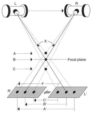
FIG. 13-26 Tomographic techniques.
As the x-ray tube moves from left to right, the film moves in the opposite direction. In the figure, points A and C lie outside the focal plane (the plane that contains the fulcrum), whereas object B lies at the center of tube/film movement. Only objects that lie in the focal plane (i.e., B) remain in sharp focus because the image of B moves exactly the same distance (B′) as the film travels (F), and thus its image remains stationary on the film. The image of point A moves more than the film (distance A′) and the image of point C less than the film (distance C′); therefore the images of both are blurred. X is the tomographic angle. The greater the tomographic angle, the thinner the tomographic layer.
• Overlying structures lie far from the focal plane
• The focal plane lies far from the film
• The long axis of the structure to be blurred is oriented perpendicular to the direction of tube travel
There are at least five types of tomographic movement: linear, circular, elliptic, hypocycloidal, and spiral (Fig. 13-27). Mechanically, the simplest tomographic motion is linear. More complex movements such as circular, elliptic, hypocycloidal, and spiral produce images without streaking artifacts common to the linear movements. Many of the more expensive panoramic units are capable of making tomographic sections of the jaws (Fig. 13-28).
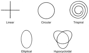
FIG. 13-27 Tomographic movements.
Linear movements, either vertical or horizontal, are mechanically simple but result in streaking artifacts. The more complex motions result in fewer streaking artifacts and sharper images.
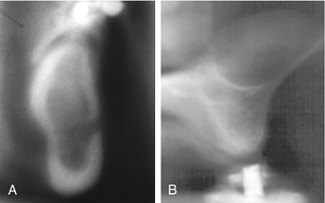
FIG. 13-28 Linear Tomographic Images Made by Panoramic Units.
A, Mandibular tomogram in the region of the mental foramen. B, Maxillary tomograms in the premolar region acquired with an Instrumentarium Orthopantomograph 100 panoramic unit. Note the dome-shaped opacity in the floor of the maxillary sinus consistent with a mucous retention phenomenon. (B, Courtesy Brad Potter, DDS, Augusta, Ga.)
Bononmo, L, Foley, D, Imhof, H, et al. Multidetector computed tomography technology: advances in imaging techniques, ed 1. London: Royal Society of Medicine Press; 2003.
Bushberg, JT, Seibert, JA, Leidholdt, EM, Jr., et al. The essential physics of medical imaging, ed 2. Baltimore: Williams & Wilkins; 2002.
Bushong, SC. Computed tomography, ed 1. New York: McGraw-Hill; 2000.
Fishman, EK, Jeffrey, RB, Jr. Multidetector CT: principles, techniques, and clinical applications, ed 1. Philadelphia: Lippincott Williams & Wilkins; 2004.
Kalender, W. Computed tomography: fundamentals, systems technology, image quality, applications, ed 2. Erlangen: Publicis Corporate Publishing; 2005.
Knollmann, F, Coakley, FV. Multislice CT: principles and protocols, ed 1. Philadelphia: Elsevier; 2006.
Marchal, G, Vogl, TJ, Heiken, JP, et al. Multidetector-row computed tomography, ed 1. Milan: Springer; 2005.
Silverman, PM. Multislice computed tomography: a practical approach to clinical protocols, ed 1. Philadelphia: Lippincott Williams & Wilkins; 2002.
Bushberg, JT, Seibert, JA, Leidholdt, EM, Jr., et al. The essential physics of medical imaging, ed 2. Baltimore: Williams & Wilkins; 2002.
Westbrook, C, Roth, CK, Talbot, J. MRI in practice, ed 3. Oxford: Blackwell Publishing; 2005.
Mettler, FA, Guiberteau, MJ. Essentials of nuclear medicine, ed 5. Philadelphia: WB Saunders; 2006.
Schiepers, C. Diagnostic nuclear medicine, ed 2. Berlin: Springer; 2006.
Sharp, PF, Gemmell, HG, Murray, AD. Practical nuclear medicine, ed 3. London: Springer-Verlag; 2005.
Wilson, MA. Nuclear medicine, ed 1. Philadelphia: Lippincott-Raven; 1998.
Brant, WE. Ultrasound, ed 1. Philadelphia: Lippincott Williams & Wilkins; 2001.
Emshoff, R, Bertram, S, Strobl, H. Ultrasonographic cross-sectional characteristics of muscles of the head and neck. Oral Surg Oral Med Oral Pathol Oral Radiol Endod. 1999;87:93–106.
Goldman LW, Fowlkes JB, eds. Categorical course in diagnostic radiology physics: CT and US cross-sectional imaging. Oak Brook, Ill: RSNA Publications, 2000.
Middleton, WD, Kurtz, AB, Hertzberg, BA. Ultrasound: the requisites, ed 2. St. Louis: Mosby; 2004.
Shimizu, M, Okamura, K, Yoshiura, K, et al. Sonographic diagnostic criteria for screening Sjögren’s syndrome. Oral Surg Oral Med Oral Path Oral Radiol Endod. 2006;102:85–93.