Using Statistics to Predict
The ability to predict future events is becoming increasingly important in our society. We are interested in predicting who will win the football game, what the weather will be like next week, or what stocks are likely to rise in the near future. In nursing practice, as in the rest of society, the capacity to predict is crucial. For example, we need to predict the length of stay of patients with varying severity of illness, as well as the response of patients with a variety of characteristics to nursing interventions. We need to know what factors play an important role in patients’ responses to rehabilitation. One might be interested in knowing what variables were most effective in predicting a student’s score on the State Board of Nurse Examiners’ Licensure Examination.
The statistical procedure most commonly used for prediction is regression analysis. The purpose of a regression analysis is to predict or explain as much of the variance in the value of a dependent variable as possible. In some cases, the analysis is exploratory, and the focus is prediction. In others, selection of variables is based on a theoretical position, and the purpose is to develop an explanation that confirms the theoretical position.
Predictive analyses are based on probability theory rather than decision theory. Prediction is one approach to examining causal relationships between or among variables. The independent (predictor) variable or variables cause variation in the value of the dependent (outcome) variable. The goal is to determine how accurately one can predict the value of an outcome (or dependent) variable based on the value or values of one or more predictor (or independent) variables. This chapter describes some of the more common statistical procedures used for prediction. These procedures include simple linear regression, multiple regression, and discriminant analysis.
SIMPLE LINEAR REGRESSION
Simple linear regression provides a means to estimate the value of a dependent variable based on the value of an independent variable. The regression equation is a mathematical expression of a causal proposition emerging from a theoretical framework. This link between the theoretical statement and the equation should be made clear before the analysis. Simple linear regression is an effort to explain the dynamics within the scatter plot by drawing a straight line (the line of best fit) through the plotted scores. This line is drawn to best explain the linear relationship between two variables. Knowing that linear relationship, we can, with some degree of accuracy, use regression analysis to predict the value of one variable if we know the value of the other variable.
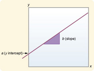
Simple linear regression is a method of determining parameters a and b. When squared deviation values are minimized, variance from the line of best fit is minimized. To understand the mathematical process, recall the algebraic equation for a straight line:
In regression analysis, the straight line is usually plotted on a graph, with the horizontal axis representing x (the independent, or predictor, variable) and the vertical axis representing y (the dependent, or predicted, variable). The value represented by the letter a is referred to as the yintercept, or the point where the regression line crosses (or intercepts) the y axis. At this point on the regression line, x = 0. The value represented by the letter b is referred to as the slope, or the coefficient of x. The slope determines the direction and angle of the regression line within the graph. The slope expresses the extent to which y changes for every 1-unit change in x.Figure 21-1 is a graph of these points.
In simple, or bivariate, regression, predictions are made in cases with two variables. The score on variable y (dependent variable) is predicted from the same subject’s known score on variable x (independent variable). The predicted score (or estimate) is referred to as ŷ (expressed y-hat) or occasionally as y′ (expressed y-prime).
No single regression line can be used to predict with complete accuracy every y value from every x value. In fact, you could draw an infinite number of lines through the scattered paired values. However, the purpose of the regression equation is to develop the line to allow the highest degree of prediction possible—the line of best fit. The procedure for developing the line of best fit is the method of least squares.
Interpretation of Results
The outcome of analysis is the regression coefficient R. When R is squared, it indicates the amount of variance in the data that is explained by the equation. A null regression hypothesis states that the population regression slope is 0, which indicates that there is no useful linear relationship between x and y. (There are regression analyses that test for nonlinear relationships.) The test statistic used to determine the significance of a regression coefficient is t. However, the test uses a different equation than the t-test used to determine significant differences between means. In determining the significance of a regression coefficient, t tends to become larger as b moves farther from zero. However, if the sum of squared deviations from regression is large, the t value will decrease. Small sample sizes also decrease the t value.
In reporting the results of a regression analysis, the equation is expressed with the calculated coefficient values. The R2 value and the t values are also documented. The format for reporting the results of regression is as follows:
The figures in parentheses are not always t values. They may be the standard error of the estimate. Therefore, the report must indicate which values are being reported. If t values are being used, the t value that indicates significance should also be reported. A t value equal to or greater than the table value (see Appendix A) indicates significance. Researchers can use these results to develop a graph that illustrates the outcome. Additionally, a table can be developed to indicate the changes that are predicted to occur in the value of y with each increase in the value of x. Names are usually given to identify the variables of x and y. In the example in which the y intercept = 3.45 and b = 8.72, a table of x and y values was developed (Table 21-1). These values are graphed in Figure 21-2.
TABLE 21-1
Predicted Values of y from Known Values of x by Regression Analysis
| Value of x | Predicted Value of y |
| 0 | 3.45 ( y intercept) |
| 1 | 12.17 ( y intercept +b) |
| 2 | 20.89 (+b) |
| 3 | 29.61 (+b) |
| 4 | 38.33 (+b) |
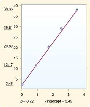
Figure 21-2 Regression line developed from values in Table 21-1.
After a regression equation has been developed, the equation is tested against a new sample to determine its accuracy in prediction, a process called cross-validation. In some studies, data are collected from a holdout sample obtained at the initial data collection period but not included in the initial regression analysis. The regression equation is then tested against this sample. Some “shrinkage” of R2 is expected because the equation was generated to best fit the sample from which it was developed. However, an equation is most useful if it maintains its ability to accurately predict across many and varied samples. The first test of an equation against a new sample should use a sample similar to the initial sample.
MULTIPLE REGRESSION
Multiple regression analyses are closely related mathematically to analysis of variance (ANOVA) models (ANOVA is described in Chapter 22); however, their focus is predicting rather than determining differences in groups. ANOVA is based on decision theory, whereas regression analysis is based on probability theory. Multiple regression is an extension of simple linear regression in which more than one independent variable is entered into the analysis. Examples of simple and multiple regression analysis results from published studies are presented in the Grove (2007) statistical workbook. The workbook can expand your understanding of regression analyses and the implications of the findings for practice.
Multicollinearity
Multicollinearity occurs when the independent variables in a multiple regression equation are strongly correlated. In nursing studies, some multicollinearity is inevitable; however, you can minimize multicollinearity by carefully selecting the independent variables. Multicollinearity does not affect predictive power (the capacity of the independent variables to predict values of the dependent variable in that specific sample); rather it causes problems related to generalizability. If multicollinearity is present, the equation will not have predictive validity. The amount of variance explained by each variable in the equation will be inflated. The b values will not remain consistent across samples when cross-validation is performed.
The first step in identifying multicollinearity is to examine the correlations among the independent variables. Therefore, you would perform multiple correlation analyses before conducting the regression analyses. The correlation matrix is carefully examined for evidence of multicollinearity. Most researchers consider multicollinearity to exist if a bivariate correlation is greater than 0.65. However, some researchers use a stronger correlation of 0.80 or greater as an indication of multicollinearity (Schroeder, 1990).
The coefficient of determination (R2), computed from a matrix of correlation coefficients, provides important information on multicollinearity. This value indicates the degree of linear dependencies among the variables. As the value of the determinant approaches zero, the degree of linear dependency increases. Thus, it is preferable that this R2 be large. Identifying the extent of multicollinearity is important when selecting regression procedures and interpreting results. Therefore, Schroeder (1990) described additional procedures that researchers use to diagnose the extent of multicollinearity.
The researcher needs to examine the extent of multicollinearity in the data as part of the analysis procedure and should report this information when the study is published. An example from Braden (1990) follows.
Types of Independent Variables Used in Regression Analyses
Variables in a regression equation can take many forms. Traditionally, as with most multivariate analyses, variables are measured at the interval level. However, researchers also use categorical or dichotomous measures (referred to as dummy variables), multiplicative terms, and transformed terms. A mixture of types of variables may be used in a single regression equation. The following discussion describes the various terms used as variables in regression equations.
Dummy Variables
To use categorical variables in regression analysis, a coding system is developed to represent group membership. Categorical variables of interest in nursing that might be used in regression analysis include gender, income, ethnicity, social status, level of education, and diagnosis. If the variable is dichotomous, such as gender, members of one category are assigned the number 1, and all others are assigned the number 0. In this case, for gender the coding could be
If the categorical variable has three values, two dummy variables are used; for example, social class could be classified as lower class, middle class, or upper class. The first dummy variable (X1) would be classified as
The second dummy variable (X2) would be classified as
The three social classes would then be specified in the equation in the following manner:
When more than three categories define the values of the variable, increased numbers of dummy variables are used. The number of dummy variables is always one less than the number of categories.
Time Coding
Time is commonly expressed in a regression equation as an interval measure. However, in some cases, codes may need to be developed for time periods. In this strategy, time is coded in a categorical form and used as an independent variable. For example, if 5 years of data were available, the following system could be used to provide dummy codes for the time variable:
Effect Coding
Effect coding is similar to dummy coding but is used when the effects of treatments are being examined by the analysis. Each group of subjects is assigned a code. The code numbers used are 1, 0, and −1. The codes are assigned in the same way as dummy codes. While using dummy codes, one category will be assigned 0; in effect coding, one group in each set will be assigned −1, one group will be assigned 1, and all others will be assigned 0 (Pedhazur, 1997).
Multiplicative Terms
The multiple regression model Y = a + b1X1 + b2X2 + b3X3 assumes that the independent variables have an additive effect on the dependent variable. In other words, each independent variable has the same relationship with the dependent variable at each value of the other independent variables. Thus, if variable X1 increased as X2 increased in lower values of X2, X1 would be expected to continue to increase at the same rate at higher values of X2. However, in some analyses, this does not prove to be the case. For example, in a study of hospice care conducted by one of the authors (Burns & Carney, 1986), minutes of care (MC) was used as the dependent variable. Duration (DUR), or number of days of care, and age (AGE) were included as independent variables. When duration was short, minutes of care increased as age increased. However, when duration was long, minutes of care decreased as age increased.
In this situation, better prediction can occur if multiplicative terms are included in the equation. In this case, the regression model takes the following form:
The last term(b3X1X2) takes the form of a multiplicative term and is the product of the first two variables (X1 multiplied by X2). This term expresses the joint effect of the two variables. For example, duration (DUR) might be expected to interact with the subject’s age (AGE). The third term shows the combined effect of the two variables (DURAGE). The example equation would then be expressed as

This procedure is similar to multivariate ANOVA, in which main effects and interaction effects are considered. Main effects are the effects of a single variable. Interaction effects are the multiplicative effects of two or more variables.
Transformed Terms
The typical regression model assumes a linear regression in which the relationship between X and Y can be illustrated on a graph as a straight line. However, in some cases, the relationship is not linear but curvilinear. A researcher can sometimes demonstrate the fact that the scores are curvilinear by graphing the values. In these cases, deviations from the regression line will be great and predictive power will be low; the F ratio will not be significant, R2 will be low, and a type II error will result. Adding another independent variable to the equation, a transformation of the original independent variable obtained by squaring the original variable, may accurately express the curvilinear relationship. This strategy improves the predictive capacity of the analysis. An example of a mathematical model that includes a squared independent variable is
This equation states that Y is related to both X and X2 in such a way that changes in Y’s values are a function of both X and X2. The nonlinearity analysis can be extended beyond the squared term to add more transformed terms; thus, values such as X3, X4, and so on can be included in the equation. Each term adds another curve in the regression line. With this strategy, complicated relationships can be modeled. However, small samples can incorrectly lead to a perfect fit. For these complex equations, the researcher needs a minimum of 30 observations per term (Cohen & Cohen, 1983). If the complex equation provides better prediction, R2 will increase and the F ratio will be significant.
Many versions of regression analyses are used in a variety of research situations. Some versions have been developed especially for situations in which some of the foregoing assumptions are violated.
The typical multiple regression equation is expressed as
The dependent variable (or predicted variable) is represented by Y in the regression equation. The independent variables (or indicators) are represented by Xi in the regression equation. The i indicates the number of independent variables in the equation. The coefficient of the independent variable, b, is a numerical value that indicates the amount of change that occurs in Y for each change in the associated X and can be reported as a b weight (based on raw scores) or a beta weight (based on Z scores).
The outcome of a multiple regression is an R2 value. For each independent variable, the significance of R2 is reported, as well as the significance of b. Regression, unlike correlation, is one-way; the independent variables can predict the values of the dependent variable, but the dependent variable cannot be used to predict the values of the independent variables. If the b value of an independent variable is not significant, that independent variable is not an effective predictor of the dependent variable when that set of independent variables is used. In this case, the researcher may remove variables with nonsignificant coefficients from the equation and repeat the analysis. This action often increases the amount of variance explained by the equation and thus raises the R2 value. To be effective predictors, independent variables selected for the analysis should have strong correlations with the dependent variable but only weak correlations with other independent variables in the equation.
The significance of an R2 value is tested with an F test. A significant F value indicates that the regression equation has effectively predicted variation in the dependent variable and that the R2 value is not a random variation from an R2 value of zero.
Results
The outcome of regression analysis is referred to as a prediction equation. This equation is similar to that described for simple linear regression except that making a prediction is more complex. Consider the following sample equation:

If duration were measured as the number of days that the patient received care, the Y intercept would be 10.6 days. (This value is not meaningful apart from the equation.) For each increase of 1 year in age, the patient would receive 0.3 days more of care. For each increase in income level, the patient would receive an additional 2.4 days of care. For each increase in coping ability measured on a scale, the patient would receive an additional 3.5 days of care. In this example, R2 = 0.51, which means that these variables explain 51% of the variance in the duration of care. The regression analysis of variance indicates that the equation is significant at a p ≤ 0.001 level. The values in parentheses are the standard deviation for that variable.
Relating these findings to real situations requires additional work. First, it is necessary to know how the variables were coded for the analysis; for example, one would need to know the range of scores on the coping scale, the income classifications, and the range of ages in the sample. Possible patient situations would then be proposed, and the duration of care would be predicted for a patient with those particular dimensions of each independent variable. For example, suppose a patient is 64 years of age, in income level 3, and in coping level 5. In this case, the patient’s predicted duration would be 10.6 + (64 × 0.3) + (3 × 2.4) + (5 × 3.5), or 54.5 days of care.
The results of a regression analysis are not expected to be sample specific. The final outcome of a regression analysis is a model from which values of the independent variables can be used to predict and perhaps explain values of the dependent variable in the population. If so, the analysis can be repeated in other samples with similar results. The equation is expected to have predictive validity. Knapp (1994) has listed the essential elements of a regression analysis that need to be included in a publication.
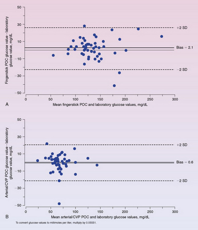
Lacara et al. (2007), all advanced practice nurses, performed a regression analysis to examine values obtained from blood for point-of-care analysis of glucose levels. Blood was often taken from different sources (e.g., fingerstick, arterial, or central venous catheter). Their objective was to examine the agreement between point-of-care and laboratory glucose values and to judge the accuracy of the point-of-care values. The researchers used a t-test to determine differences in values between each point-of-care source and the laboratory value. They used multiple regression analysis to determine if serum level of carbon dioxide, hematocrit, or mean arterial pressure significantly contributed to the difference in bias and precision for the point-of-care blood sources. They reported their results as follows.
Table 21-2 provides results of the multiple regression analysis. The authors also used Bland and Altman plots, described in Chapter 19, to depict the differences between the laboratory glucose value and the point-of-care glucose values (Figure 21-3).
TABLE 21-2
Multiple Regression Analysis of POC and Laboratory Glucose Difference Scores for Three Independent Variables
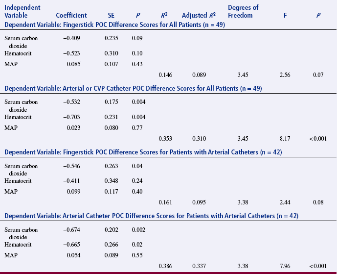
CVP, central venous pressure; MAP, mean arterial pressure; POC, point of care.
From Lacara, T., Domagtoy, C., Lickliter, D., Quattrocchi, K. Snipes, L., Kuszaj, J., et al. (2007). Comparison of point-of-care and laboratory glucose analysis in critically ill patients. American Journal of Critical Care, 16(4), 341.
Cross-Validation
To determine the accuracy of the prediction, the predicted values are compared with actual values obtained from a new sample of subjects or values from a sample obtained at the time of the original data collection but held out from the initial analysis. This analysis is conducted on the difference scores between predicted values and the means of actual values. Thus, in the new sample, the number of days of care for all patients 64 years of age, in income level 3, and in coping level 5 is averaged, and the mean is compared with 54.5 days of care. Each possible case within the new sample is compared in this manner. An R2 is obtained on the new sample and compared with the R2 of the original sample. In most cases, R2 will be lower in the new sample, because the original equation was developed to most precisely predict scores in the original sample. This phenomenon is referred to as shrinkage of R2. Shrinkage of R2 is greater in small samples and when multicollinearity is great.
DISCRIMINANT ANALYSIS
Discriminant analysis allows the researcher to identify characteristics associated with group membership and to predict group membership. The dependent variable is membership in a particular group. The independent variables (discriminating variables) measure characteristics on which the groups are expected to differ. Discriminant analysis is closely related to both factor analysis and regression analysis. However, in discriminant analysis, the dependent variable values are categorical in form. Each value of the dependent variable is considered a group. When the dependent variable is dichotomous, the researcher performs multiple regression. However, when more than two groups are involved, analysis becomes much more complex. The dependent variable in discriminant analysis is referred to as the discriminant function. It is equivalent in many ways to a factor (Edens, 1987).
Two similar data sets are required for complete analysis. The first data set must contain measures on all the variables to be included in the analysis and the group membership of each subject. The purpose of analysis of the first data set is to identify variables that most effectively discriminate between groups. Selection of variables for the analysis is based on the researcher’s expectation that they will be effective in this regard. The researcher then tests the variables selected for the discriminant function on a second set of data to determine their effectiveness in predicting group membership (Edens, 1987).
SUMMARY
• Predictive analyses are based on probability theory rather than decision theory. Prediction is one approach to examining causal relationships between or among variables.
• The independent (predictor) variable or variables cause variation in the value of the dependent (outcome) variable.
• The purpose of a regression analysis is to predict or explain as much of the variance in the value of the dependent variable as possible.
• Simple linear regression provides a means to estimate the value of a dependent variable based on the value of an independent variable.
• Multiple regression analysis is an extension of simple linear regression in which more than one independent variable is entered into the analysis.
• Multicollinearity occurs when the independent variables in a multiple regression equation are strongly correlated.
• The outcome of regression analysis is referred to as a prediction equation. The final outcome of a regression analysis is a model from which values of the independent variables can be used to predict and perhaps explain values of the dependent variable in the population.
• Discriminant analysis allows the researcher to identify characteristics associated with group membership and to predict group membership.
REFERENCES
Braden, C.J. A test of the self-help model: Learned response to chronic illness experience. Nursing Research. 1990;39(1):42–47.
Burns, N., Carney, K. Patterns of hospice care: The RN role. Hospice Journal. 1986;2(1):37–62.
Cohen, J., Cohen, P. Applied multiple regression/correlation analysis for the behavioral sciences. Hillsdale, NJ: Lawrence Erlbaum, 1983.
Edens, G.E. Discriminant analysis. Nursing Research. 1987;36(4):257–262.
Gordon, R. Issues in multiple regression. American Journal of Sociology. 1968;73(5):592–616.
Grove, S.K. Statistics for health care research: A practical workbook. Philadelphia: Saunders, 2007.
Knapp, T.R. Regression analyses: What to report. Nursing Research. 1994;43(3):187–189.
Lacara, T., Domagtoy, C., Lickliter, D., Quattrocchi, K., Snipes, L., Kuszaj, J., et al. Comparison of point-of-care and laboratory glucose analysis in critically ill patients. American Journal of Critical Care. 2007;16(4):336–346.
Pedhazur, E.J. Multiple regression in behavioral research. Philadelphia: Harcourt Brace, 1997.
Schroeder, M.A. Diagnosing and dealing with multicollinearity. Western Journal of Nursing Research. 1990;12(2):175–187.