Chapter 36

Regulation of Gene Expression

Genomics, Proteomics and Metabolomics

Andrew R. Pitt and Walter Kolch

Learning objectives

After reading this chapter you should be able to:

Describe what the terms genomics, transcriptomics, proteomics, and metabolomics mean.

Discuss the differences between the -omics methods and their particular challenges.

Describe the structure of a gene and the regulation of gene transcription.

Give several examples of methods used in genomics and transcriptomics.

Give examples of methods used in proteomics.

Describe methods used in metabolomics.

Discuss biomarkers.

Introduction

The human genome is organized into 46 chromosomes consisting of 22 pairs of autosomal chromosomes, which are shared by both sexes, and the sex-determining chromosomes, X and Y. One set of autosomal chromosomes is derived from each parent. One X chromosome is contributed by the mother and another, either X or Y from the father. Most mammalian genes consist of multiple exons, which are the parts that eventually constitute the mature mRNA, and introns, which separate the exons and are removed from the primary transcript by splicing.

Many of the complex biological functions are generated by interaction between genes rather than by individual genes

Surprisingly, the 3 billion bases of the human genome only harbor 22,000–24,000 protein-coding genes. This is only about four times the number of genes of yeast and twice as many as the fruit fly Drosophila melanogaster, and less than many plants. Thus, many of the complex biological functions that characterize humans are generated by combinatorial interaction between genes rather than by individual genes being responsible for a specific function. This insight has replaced the dogma of one gene encoding one protein with one function. Mammalian cells use alternative splicing and alternative gene promoters to produce 4–6 different mRNA from a single gene, so that the number of protein-coding mRNAs, the transcriptome, may be as large as 100,000.

Post-translational modifications add further levels of complexity

This complexity is further augmented at the protein level by post-translational modifications and targeted proteolysis that could generate an estimated 500,000–1,000,000 functionally different protein entities, which comprise the proteome. An estimated 10–15% of these proteins function in metabolism, which collectively describes the processes used to provide energy and the basic low-molecular-weight building blocks of cells, such as amino acids, fatty acids and sugars. It also includes the processes that convert exogenous substances such as drugs or environmental chemicals.

The human metabolome database (www.hmdb.ca/) currently contains >40,000 entries. The real size of the metabolome is unknown, but is expected to increase with the number of environmental substances an organism is exposed to. The relationship between the different -omes is depicted in Figure 36.1.

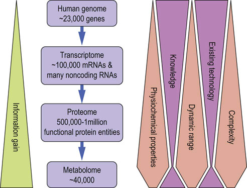
Fig. 36.1 Relationship between the -omics.
Complexity, diversity in physicochemical properties, and dynamic range increase as we move from genes to transcripts and proteins, but may decrease again at the level of metabolites. This presents a huge technologic challenge, but also represents a rich source of information gain, especially if the different -omics disciplines can be integrated into a common view.

Studies of genome, transcriptome, proteome and metabolome pose different challenges

The genome and transcriptome consist entirely of the nucleic acids DNA and RNA, respectively. Their uniform physicochemical properties have enabled efficient and ever cheaper methods for amplification, synthesis, sequencing and highly multiplexed analysis. The proteome and metabolome pose much bigger analytical challenges as they consist of molecules with widely different physicochemical properties and highly variable abundance. For instance, the concentration of proteins in human serum spans 12 orders of magnitude, while under normal conditions genes are equally abundant. The genome is relatively static, whereas the transcriptome and proteome are more dynamic and can change quickly in response to internal and external cues. The most pronounced dynamic responses may manifest themselves in the metabolome as it directly reflects the interactions between organism and environment. Thus, the complexity increases as we move from the genome to the transcriptome, proteome and metabolome, while our knowledge decreases. The analysis of all -omics data requires large and sophisticated bioinformatics resources, and also has stimulated the development of systems biology, which uses mathematical and computational modeling to interpret the functional information about biological processes contained in these data.

Genomics

Genome analysis provides a way to predict the probability of a condition, but without providing information whether and when this probability will manifest itself

The ‘whether and when’ information can better be gained from the transcriptome, proteome and metabolome. They give a dynamic picture of the current state of an organism, and lend themselves to monitor changes in that state, e.g. during disease progression or treatment. Thus, the information provided by the -omics technologies is complementary, and their use for diagnostic purposes is mainly limited by the complexity of the equipment and analysis. Genomics and transcriptomics are making their way into the clinical laboratory, and are poised to become part of routine diagnostics in the next few years.

Many diseases have an inheritable genetic component

Many diseases are caused by genetic aberrations and many more manifest a genetic predisposition or component. The Online Mendelian Inheritance in Man (OMIM) database (www.omim.org/) currently lists more than 2,800 gene mutations that are associated with >4,700 phenotypes which cause or predispose to disease. These numbers suggest that many diseases are caused by mutations in single genes, and that many more have an inheritable genetic component. Thus, the genome holds a rich source of information about our physiology and pathophysiology. We now have a broad arsenal of techniques for genome analysis at our disposal, which allow the detection of gross abnormalities down to single nucleotide changes, and which are increasingly being used for clinical diagnostics.

Advanced concept box The human genome project

The Human Genome Project (HGP) officially began in 1990 and culminated with the deposition of the completed sequence into public databases in 2003. However, in-depth analysis and interpretation will go on for much longer. The HGP was unique in several ways. It was the first global life science project, being coordinated by the Department of Energy and the National Institutes of Health (USA). The Wellcome Trust (UK) became a major partner in 1992, and further significant contributions were made by Japan, France, Germany, China, and other countries. More than 2800 scientists from 20 institutions around the world contributed to the paper describing the finished sequence in 2004. It also was conducted on an industrial scale with industrial-style logistics and organization. In fact, the HGP received competition from Celera Genomics, a private company founded in 1998, and the first draft sequences of the human genome were published in two parallel papers in 2001. The HGP used a ‘clone-by-clone’ approach where the genome was cloned first and then these large clones were divided into smaller portions and sequenced. Celera followed a fundamentally different strategy, shotgun sequencing, where the whole genome is broken up into small pieces that can be sequenced directly with the full sequence being assembled afterwards. This approach is much faster but less reliable in producing continuous sequences, and much less able to mend gaps in the assembled sequence. The 2001 draft genomes estimated the existence of 30,000–35,000 genes. The refined HGP 2003 sequence confirmed 19,599 protein-coding genes and identified another 2188 DNA predicted genes, a surprisingly low number. They are contained in 2.85 billion nucleotides covering more than 99% of the euchromatin, i.e. gene-containing DNA. Many thousands of genomes have been sequenced since then, and the human reference genome is constantly updated. As by 2010 there are only ~250 gaps compared to the 150,000 in the draft sequence, and the current sequence is extremely accurate. Genome sequences are accessible publicly through all major nucleotide databases.

Karyotyping, comparative genome hybridization (CGH), chromosomal microarray analysis (CMA) and fluorescence in situ hybridization (FISH)

Karyotyping assesses the general chromosomal architecture

Early successes of exploiting genome information for the diagnosis of human disease was the discovery of trisomy 21 as the cause of Down syndrome in 1959, and the discovery of the Philadelphia chromosome as associated with chronic myelogenous leukemia (CML) in 1960. Since then karyotyping has identified a large number of chromosomal aberrations, including amplifications, deletions and translocations, especially in tumors. The method is based on simple staining of chromosome spreads by Giemsa or other stains which reveal a banding pattern characteristic for each chromosome that is visible through the light microscope. Although it only reveals crude information such as number, shapes and gross alterations of general chromosomal architecture, it is still a mainstay of clinical genetic analysis.

Comparative genome hybridization compares two genomes of interest

A refinement of karyotyping is comparative genome hybridization (CGH). The principle of CGH is to compare two genomes of interest, usually a diseased against a normal control genome. The genomes that are to be compared are labeled with two different fluorescent dyes. The fluorescently labeled DNAs are then hybridized to a spread of normal chromosomes and evaluated by quantitative image analysis (Fig. 36.2). As fluorescence has a large dynamic range (i.e. the relationship between fluorescence intensity and concentration of the probe is linear over a wide range), CGH can detect regional gains or losses in chromosomes with much higher accuracy and resolution than conventional karyotyping. Losses of 5–10 megabases (Mb) and amplifications of <1 Mb are detectable by CGH. However, balanced changes, such as inversions or balanced translocations, escape detection as they do not change the copy number and hybridization intensity.

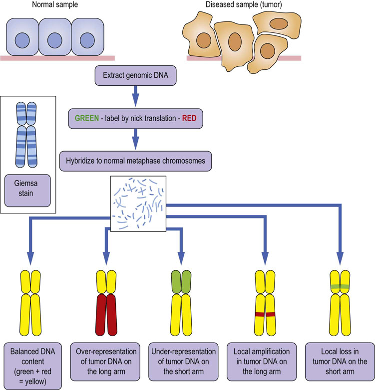
Fig. 36.2 Principles of comparative genome hybridization (CGH).
Genomic DNA is isolated from a normal and a diseased sample (here, from a tumor) to be compared. The DNA is labeled by nick translation with green or red fluorescent dyes, and hybridized to a normal chromosome spread. If the DNA content between samples is balanced, equal amounts of the control (green) and tumor (red) DNA will hybridize, resulting in a yellow color. Global or local amplifications or losses of genetic material will reveal themselves by a color imbalance.

In chromosomal microarray analysis the labeled DNA is hybridized to an array of oligonucleotides

Further improvements in resolution are afforded by chromosomal microarray analysis (CMA). In this method, the labeled DNA is hybridized to an array of oligonucleotides. Modern oligonucleotide synthesis and array manufacturing can produce arrays containing many million oligonucleotides on chips of the size of a microscope slide. By choosing the oligonucleotides so that they cover the region of interest to an equal extent, a very high resolution can be achieved, allowing the detection of copy number changes at the level of 5–10 kb in the human genome. CMA is used in prenatal screening for the detection of chromosomal defects. As the probe DNA can be amplified by the polymerase chain reaction (PCR; Fig. 36.3), only minute amounts of starting material are required. Notably, neither CGH nor CMA provides information about the ploidy. As long as the DNA content is balanced and carries no further aberrations, a tetraploid genome would be indistinguishable from a diploid genome.

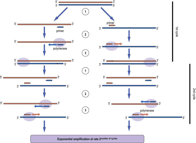
Fig. 36.3 Polymerase chain reaction (PCR).
This method is widely used for the amplification of DNA and RNA. The nucleic acid template is heat-denatured and specific primers are annealed by lowering the temperature (step 1). The primers are extended using reverse transcriptase if the template is RNA, or a DNA polymerase if the template is DNA (step 2). The result is a double-stranded product (step 3), which is heat denatured so that the cycle can start again. Typically, between 25 and 35 cycles are used. The amplification is exponential, and hence PCR enables us to analyze minute amounts of DNA or RNA down to the single cell level. The use of heat-stable and high-fidelity DNA polymerases permits amplification of fragments up to several thousand base pairs long. Many variations of PCR have been developed for a wide range of applications, such as molecular cloning, site-directed mutagenesis, generation of labeled probes for hybridization experiments, quantitation of RNA expression, DNA sequencing, genotyping, and many others.

Fluorescence in situ hybridization can be used when the gene in question is known

If the gene of interest is known, the respective recombinant DNA can be labeled and used as a probe on chromosome spreads. This method, called fluorescence in situ hybridization (FISH), can detect gene amplifications, deletions and chromosomal translocations. Using different colored fluorescent labels, several genes can be stained simultaneously.

Gene mutations can be studied by sequencing

Efforts to find individual disease genes were hampered by our insufficient knowledge of the genome and by the lack of high-resolution mapping methods. This situation dramatically changed with the completion of the human genome sequence in 2003 and the rapid development of novel technologies, called next-generation sequencing (NGS), which made sequencing very fast and affordable.

Four principles of DNA sequencing

There are four principles of DNA sequencing. (i) The Maxam–Gilbert method uses chemicals to cleave the DNA at specific bases and then separate the fragments on high-resolution gels, allowing the sequence to be read from the size of the fragments. (ii) The Sanger method uses a polymerase to synthesize DNA in the presence of small amounts of chain-terminating nucleotides (Fig. 36.4). This and the Maxam–Gilbert method were the first successful DNA sequencing techniques. While the latter has become obsolete, the Sanger method is still widely used. (iii) The extension of the complementary DNA strand is measured when a matching nucleotide is added. (iv) The ligation of a synthetic oligonucleotide to the DNA target to be sequenced, which only occurs when a nucleotide pair in the oligonucleotide matches the sequence of the target DNA at the correct position, is monitored. Variations of methods ii–iv are incorporated in NGS workflows.

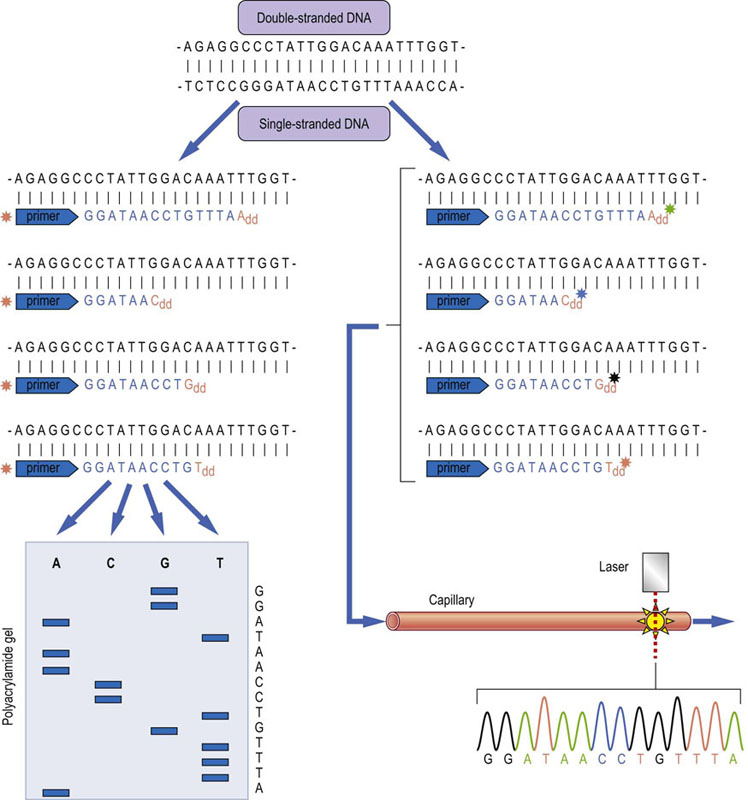
Fig. 36.4 DNA sequencing using Sanger's chain termination method.
Double-stranded DNA is heat-denatured to generate single-stranded DNA. Primers (usually hexamers of random sequence) are annealed to generate random initiation sites for DNA synthesis, which is carried out in the presence of DNA polymerase, deoxynucleotides (dNTPs) and small amounts of dideoxynucleotides (ddNTPs). The ddNTPs lack the 3'-hydroxyl group which is required for DNA strand elongation. They terminate the synthesis, leading to fragments of different sizes, each ending a specific nucleotide. These fragments can be separated by polyacrylamide gel electrophoresis and the sequence read from the ‘ladder’ of fragments on the gel. To visualize the fragments, either the DNA can be labeled by adding in radioactive or fluorescent dNTPs, or the primers can be labeled (as indicated in the figure) with a fluorescent dye. Using ddNTPs labeled with different dyes permits all four reactions being mixed together and separated by capillary electrophoresis. Online laser detection enables direct reading of the sequence. This ‘capillary DNA sequencing’ gives longer reads than gels, permits multiplexing, and high throughput. It was the method used for most of the sequencing in the Human Genome Project.

There are several NGS methods using different ways to read the DNA sequence

All NGS methods share the principle of conducting many millions of parallel sequencing reactions in microscopic compartments on arrays or nanobeads. These sequence pieces are assembled into complete genome sequences using sophisticated bioinformatics methods. While the first human genome sequence cost $3 billion and took more than10 years to complete, thanks to NGS we now can sequence a human genome in a single day for ~$1000. Thus, NGS has enabled the large-scale hunt for gene mutations by direct sequencing. Notable examples of such projects are the Cancer Genome Projects executed by the Wellcome Trust Sanger Centre in the UK and the US National Cancer Institute. The aim of these projects is to establish a systematic map of mutations in cancer and utilize this map for risk stratification, early diagnosis and choice of the best treatment in patients.

Single nucleotide polymorphisms (SNPs) are useful in identification and assessment of disease risk

Genomes in a population vary slightly by small changes, most often just concerning single nucleotides, called single nucleotide polymorphisms (SNPs). The most common way to examine SNPs is by direct sequencing or array-based methods. For the first method, DNA is usually amplified by PCR and then sequenced. For the second method, oligonucleotide arrays containing all possible permutations of SNPs are probed with genomic DNA, so that successful hybridization only occurs when the DNA sequences match exactly.

Systematic SNP mapping has proven useful in studying genetic identity and inheritance, and also in the identification and risk assessment of genetic diseases

The initial human genome sequences yielded ca. 2.5 million SNPs, while by 2012 more than 180 million SNPs were known. The International HapMap Project (www.hapmap.org) systematically catalogues genetic variations based on large-scale SNP analysis in 270 humans of African, Chinese, Japanese and Caucasian origin.

Genome-wide association studies (GWAS) try linking the frequency of SNPs to disease risks

Although GWAS studies have discovered new genes involved in diseases like Crohn's disease or age-related macular degeneration, the typically low risk associated with individual SNPs hampers such correlations, especially in multigenetic diseases. There is much debate how feasible it is to overcome this limitation by examining very large cohorts.

Epigenetic changes are heritable traits not reflected in the DNA sequence

Although the genome as defined by its DNA sequence is commonly viewed as the hereditary material, there are also other heritable traits that are not reflected by changes in the DNA sequence

These traits are called epigenetic changes (see also Chapter 35 and Box on p. 461). They comprise histone modifications such as acetylation and methylation that affect chromatin structure. Another modification is methylation of the DNA itself, which occurs at the N5 position of cytosines, typically in the context of the sequence CpG. Methylation of CpG clusters, so-called CpG islands, in gene promoters can shut down the expression of a gene. These methylation patterns can be heritable by a poorly understood process called genomic imprinting (Chapter 35). Aberrations in gene methylation patterns can cause diseases and are common in human tumors, often serving to silence the expression of tumor suppressor genes.

The mapping of promoter methylation patterns is very important

The most common methods to analyze DNA methylation rely on the fact that bisulfite converts cytosine residues into uracil, but leaves 5-methylcytosine intact (Fig. 36.5). This change in the DNA sequence can be detected by several methods, including DNA sequencing of the treated versus untreated DNA, differential hybridization of oligonucleotides that specifically detect either the mutated or unchanged DNA, or array-based methods. The latter methods, similar to SNP analysis, also rely on differential hybridization to find bisulfite-induced changes in the DNA, but due to the ability to put millions of oligonucleotide probes on an array, are able to interrogate large numbers of methylation patterns simultaneously. The main limitations are the possibility that bisulfite modification may be incomplete, giving rise to false positives, and the severe general DNA degradation that occurs during the harsh conditions of bisulfite modification. Some new NGS methods can detect DNA methylation directly, and this will accelerate progress in epigenomics. The epigenome is more variable between individuals than the genome. Hence it will require a greater effort to map it systematically, but also holds more individual information that can be useful for designing personal medicine approaches.

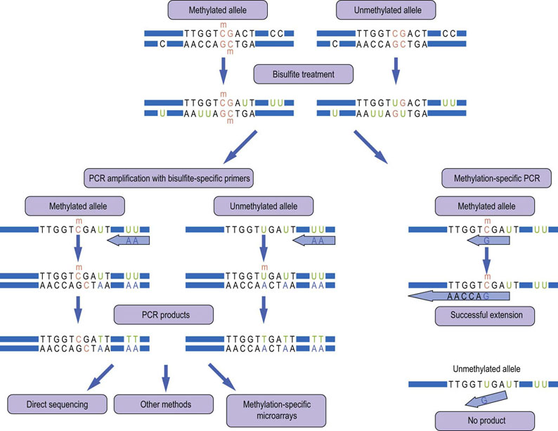
Fig. 36.5 Analysis of DNA methylation.
DNA methylation typically occurs on cytosine in the context of ‘CpG islands’ (colored orange), which are enriched in the promoter regions of genes. Bisulfite converts cytosine residues to uracil, but leaves 5-methylcytosine residues unaffected. This causes changes in the DNA sequence that can be detected in various ways. Many methods use a PCR amplification step with primers that will selectively hybridize to the modified DNA (left panel). The PCR products have characteristic sequence changes where the unmodified cytosine-guanosine base pairs are replaced by thymidine-adenosine, whereas the original sequence is maintained when the cytosine was methylated. There are many methods to analyze these PCR products. The most common are direct sequencing or hybridization to a microarray that contains oligonucleotides representing all permutations of the expected changes. Another common method is methylation-specific PCR (MSP) where the primer is designed so that it can only hybridize and extend if the cytosine was methylated and hence preserved during bisulfite treatment.

Gene expression and transcriptomics

The transcriptome represents the complement of RNAs that is transcribed from the genome

The transcription of a gene yields an average of 4–6 mRNA variants, which are translated into different proteins. The largest part of the transcriptome consists of noncoding RNAs which fulfill important structural and regulatory functions.

The transcriptome is naturally more dynamic than the genome and may differ widely between different cell types, tissues and different conditions. Genes represent the DNA sequences that correspond to functionally distinguishable units of inheritance. This definition goes back to experiments performed by Gregor Mendel, the father of genetics, in the 1860s, who showed that the color of pea plants is inherited as discrete genetic units. About 100 years later Marshall Nirenberg defined a simple relationship, i.e. ‘Gene makes RNA makes protein’, which anchored the concept that genes encode the information to make proteins and RNA is the messenger that transports that information (hence the name mRNA). It has turned out that each step is highly regulated and diversified.

Humans possess only approximately 23,000 protein-coding genes, which, however, give rise to an average of 4–6 mRNA transcripts generated by differential splicing, RNA editing and alternative promoter usage

The translation of these mRNAs into proteins (Chapter 34) is also a highly regulated process, so that no direct general correlations between mRNA expression and protein concentrations can be drawn. Protein-coding genes only constitute 1–2% of the human genome sequence, and the assumption that most transcripts originate from genes, has recently been superseded by the discovery that more than 80% of the genome can be transcribed. While some of these non-coding RNAs serve structural functions, e.g. as part of ribosomes, the large majority regulates gene transcription, mRNA processing, mRNA stability and protein translation (see Advanced Concept Box above). Thus, the largest part of the transcriptome seems dedicated to regulatory functions, and these regulatory RNAs also can be transcribed from portions of protein-encoding genes. Thus, the concept what constitutes a gene is likely due for revision in the coming years.

Advanced concept box NON-CODING RNAs (ncRNAs)

Non-coding RNAs (ncRNAs) is a summary name for RNAs which do not encode proteins. They comprise abundant species such as transfer RNAs and ribosomal RNAs, which are involved in protein translation. Several ncRNAs function as molecular guides that participate in processes which require sequence-specific recognition, such as RNA splicing or telomere maintenance. However, the vast majority of ncRNAs seems to have regulatory functions in gene expression. The call to fame came with the award of the Nobel Prize to Andrew Fire and Craig Mello in 2006 ‘for their discovery of RNA interference – gene silencing by double-stranded RNA’. These small interfering (si) RNAs are part of an enzyme complex that targets and cleaves mRNAs with high specificity conferred by the siRNA sequence. siRNAs have now become a powerful tool in the arsenal of the molecular biologist to downregulate the expression of selected mRNAs with high specificity and efficiency. Micro RNAs (miRNAs) are also small RNAs that are either transcribed under control of their own promoter or often also as part of introns in protein-coding genes. They originate from longer transcripts and are more extensively processed than siRNAs. Functionally, an important distinction is that siRNAs are very specific, requiring a perfect match to their targets, while miRNAs have imperfect sequence recognition and therefore act upon a larger number of targets, often regulating whole sets of genes. Another difference is that siRNAs induce mRNA degradation, while miRNAs can also prevent mRNA translation. The human genome encodes >1000 miRNAs, which may regulate as much as 60% of genes, thus playing a major role in the control of gene expression. Due to their pleiotropic targeting, miRNAs can affect whole programs of gene expression, and aberrant miRNA expression has been implicated in many human diseases, including cancer, obesity and cardiovascular disease.

Gene structure and gene expression

Genes consist of promoter regions, exons and introns. The promoter regulates transcription, while exons are the constituents of mRNAs

Protein-coding genes typically consist of a promoter region that contains the transcriptional start site and participates in the control of transcription, and exons and introns (Fig. 36.6). Introns are removed from the primary transcript by splicing and the mature mRNA only contains the exons. The role of introns is not clear, but they can contain regulatory sequences, including alternative promoters that can modulate gene expression. The usage of alternative promoters and alternative splicing increase the protein variants that a gene can encode.

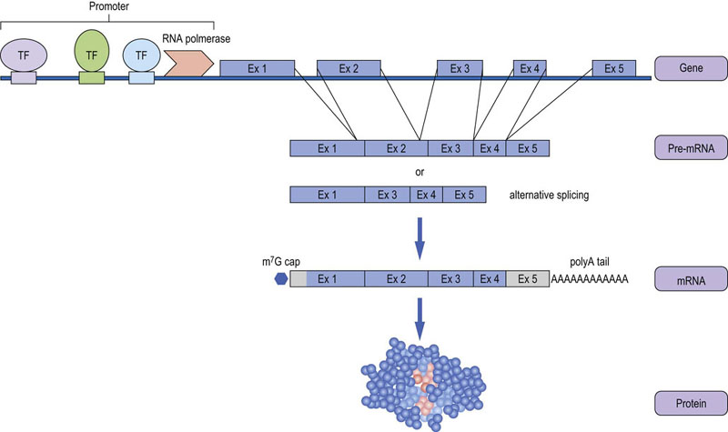
Fig. 36.6 Structure and transcription of a protein-coding gene.
Protein-coding genes are organized in exons and introns. Gene transcription is controlled by transcription factors (TFs), which bind to specific sequence elements in the gene promoter and regulate the ability of RNA polymerase to transcribe, i.e. copy, the DNA sequence of the gene into RNA. The transcribed RNA is processed into the mature messenger RNA (mRNA) by removal of the introns, addition of a polyadenyl tail at the 3'-end and a 7-methylguanosine (m⁷G) cap at the 5'-end, which mediates the binding to ribosomes and translation into protein. Untranslated exons and parts of exons are depicted in grey. Most genes produce alternatively-spliced mRNAs where different exons are included.

Some genes produce up to 20 differently spliced mRNAs, with an average estimate of ~5 transcripts per human gene

The further maturation of mRNA involves addition of a polyA tail at the 3′-end for nuclear export, and addition of a 7-methylguanylate cap at the 5′-end which is required for efficient interaction with the ribosome. The mature mRNA regions typically contain other control elements in the untranslated regions that regulate binding to ribosomes and efficiency of translation. Protein translation is explained in Chapter 34. Hence, this chapter only discusses the principles of transcriptional regulation.

Gene promoters typically have two elements: (i) a binding site for the RNA polymerase complex, which reads the DNA gene sequence and synthesizes a complementary RNA from it; and (ii) one or more binding sites for transcription factors (TFs), which modulate the transcription rate. TFs are modular proteins consisting of separable DNA binding and transactivation domains that regulate the transcriptional activity of RNA polymerase (Chapter 35). The DNA, binding domains recognize short nucleotide sequences. According to their effects on transcription, they are classified as enhancers or repressors. TFs consisting of only DNA-binding domains act as repressors as they occupy binding sites without being able to stimulate transcription. Conversely, TFs that only contain transactivation domains act as coregulators that rely on interactions with other DNA-binding proteins to regulate transcription. Binding sites that confer responses to specific stimuli or hormones are often called response elements, e.g. estrogen response element (Chapter 35). Enhancers and repressors are often located in the gene promoter, but also in introns or even far upstream or downstream of a gene as they can act over long distances. These remote effects are mediated by the yet ill-understood three-dimensional arrangement of DNA that can spatially colacate factors bound to distant sites on a linear DNA molecule.

TFs can affect transcription directly by controlling the function of RNA polymerase, or indirectly by affecting the chromatin structure

Transcription can only proceed when histones are acetylated and chromatin is in the open conformation permissive for transcription. Thus, many TFs associate with histone-modifying enzymes that change chromatin structure to either facilitate or repress transcription. TF function itself is controlled by intricate cellular signal transduction networks that process external signals, such as stimulation by growth factors, hormones and other extracellular cues, into changes of TF activities. Such changes are often conferred by phosphorylation, which can regulate the nuclear localization of TFs, their ability to bind to DNA, or their regulation of RNA polymerase activity. The presence of different TF-binding sites in a gene promoter further confers combinatorial regulation. As TFs represent more than 10% of all human genes, this multilayered type of control ensures that gene transcription can be finely adjusted in a highly versatile way to specific cellular states and environmental requirements.

Studying gene transcription by gene (micro)arrays and RNA sequencing

Methods for studying global transcription are now well established. Gene (micro)arrays contain several million DNA spots arranged on a slide in a defined order (Fig. 36.7). Modern arrays use synthetic oligonucleotides, which can be either prefabricated and deposited on the chip or synthesized directly on the chip surface. Usually several oligonucleotides are used per gene. They are carefully designed based on genome sequence information to represent unique sequences suitable for the unambiguous identification of specific RNA transcripts. Today's high-density arrays contain enough data points to survey the transcription of all human genes, map exon content and splice variants of mRNAs. Non-coding RNAs such as siRNAs and miRNAs also can be included. The arrays are hybridized with complementary RNA (cRNA) probes corresponding to the RNA transcripts isolated from the cells or tissues that are to be compared. The probes are made from isolated RNAs by copying them first into cDNA using reverse transcriptase, a polymerase that can synthesize DNA from RNA templates. The resulting complementary DNA (cDNA) is transcribed back into cRNA, as RNA hybridizes stronger to the DNA oligonucleotides on the array than cDNA would. During cRNA synthesis, modified nucleotides are incorporated that are labeled with fluorescent dyes or tags, such as biotin, which can easily be detected after hybridization of the cRNA probes to the array. After hybridization and washing off unbound probes, the array is scanned and the hybridization intensities are compared using statistical and bioinformatic analysis. The results allow a relative quantitation of changes in transcript abundances between two samples or different timepoints. Thanks to a common convention for reporting microarray experiments, called Minimal Information for the Annotation of Microarray Experiments (MIAME), array results from different experiments can be compared, and public gene array databases are a valuable source for further analysis. Gene array analysis is already being used for clinical applications. For instance, patterns of gene transcription in breast cancers have been developed into tests for assessing the risk of recurrence and the potential benefit of chemotherapy.

Fig. 36.7 The workflow of a gene (micro)array experiment.
A two-color array experiment comparing normal and cancer cells is shown as an example. See text for details. A common way to display results is heatmaps, where increasing intensities of reds and greens indicate up- and downregulated genes, respectively, while black means no change. C, cancer cells; N, normal cells. The figure is modified from http://en.wikipedia.org/wiki/DNA_microarray.

Transcriptome analysis also can be performed by direct sequencing, once the RNAs have been converted to cDNAs. The advances in rapid and cheap DNA sequencing methods permit every transcript to be sequenced multiple times. These ‘deep sequencing’ methods not only unambiguously identify the transcripts and splice forms but also allow the direct counting of transcripts over the whole dynamic range of RNA expression, resulting in absolute transcript numbers rather than relative comparisons. Thus, the sequencing methods, dubbed RNA seq, are quickly becoming attractive alternatives to array-based transcriptomics methods.

ChIP-on-chip technique combines chromatin immunoprecipitation with microarray technology

Mapping of the occupancy of transcription-factor-binding sites can reveal which genes are likely to be regulated by these factors

Our ability to survey the transcription of all known human genes poses the question which TFs are controlling the observed transcriptional patterns. The human genome contains many thousands of binding sites for any given TF, but only a small fraction of these binding sites actually is occupied by TFs and involved in the regulation of gene transcription. Thus, the systematic mapping of the occupancy of TF-binding sites can reveal which genes are actually regulated by which TFs. The techniques developed for this (Fig. 36.8) combine chromatin immunoprecipitation (ChIP) with microarray technology (chip) or DNA sequencing, and are called ChIP-on-chip or ChIP-seq.

Fig. 36.8 ChIP-on-chip analysis.
See text for details. POI (protein-of-interest). The figure has been modified from http://en.wikipedia.org/wiki/Image:ChIP-on-chip_wet-lab.png.

ChIP involves the covalent crosslinking of proteins to the DNA they are bound to by formaldehyde treatment of living cells. Then, the DNA is purified and fragmented into small (0.2–1 kb) pieces by ultrasound sonication. These DNA fragments are isolated by immunoprecipitating the crosslinked protein with a specific antibody. The associated DNA is then eluted and identified by PCR with specific primers that amplify the DNA region one wants to examine. This method assesses one binding site at a time and requires a hypothesis suggesting which site(s) should be examined. The identification of the associated DNA, however, can be massively multiplexed by using DNA microarrays for detection that represent the whole or large parts of the genome. Similarly, as discussed above, as alternative to gene microarrays, the associated DNA can be identified by sequencing.

ChIP-on-chip and ChIP-seq are powerful and informative techniques allowing the correlation of TF binding with transcriptional activity. The ChIP techniques can be used to study any protein that interacts with DNA, including proteins involved in DNA replication, DNA repair and chromatin modification. Success is critically dependent on the quality and specificity of the antibodies used, as the amounts of co-immunoprecipitated DNA are very small, and there is no other separation step than the specificity provided by the antibody.

Proteomics

Proteomics is the study of the protein complement of a cell; the protein equivalent of the transcriptome or genome

The word ‘proteome’ was coined by Marc Wilkins in a talk in Siena in 1994. Wilkins defined the proteome as the protein complement of a cell, the protein equivalent of the transcriptome or genome. Since that time the study of the proteome, called proteomics, has evolved into a number of different themes encompassing many areas of protein science.

Proteomics is possibly the most complex of all the -omics sciences but is also likely to be the most informative, since proteins are the functional entities in the cell, and virtually no biological process takes place without the participation of a protein. Among their many roles, they are responsible for the structural organization of the cell, as they make up the cytoskeleton, the control of membrane transport (Chapter 8) and energy generation. Hence, an understanding of the proteome will be necessary to understand how biology works.

Initially, proteomics concentrated on cataloguing the proteins contained in an organelle, cell, tissue or organism, in the process validating the existence of the predicted genes in the genome. This rapidly evolved into comparative proteomics, where the protein profiles from two or more samples were compared to identify quantitative differences that could be responsible for the observed phenotype: for example, from diseased versus healthy cells or looking at changes induced by drug treatment. Now, proteomics also includes the study of post-translational modifications of individual proteins, the make-up and dynamics of protein complexes, the mapping of networks of interactions between proteins, and the identification of biomarkers in disease. Quantitative proteomics has become a robust tool, and even absolute quantification is relatively routine now.

Proteomics poses several challenges

It quickly became apparent that the complexity of the proteome would be a major obstacle to achieving Wilkins' initial ideal of looking at all the proteins in a cell or organism at the same time.

While the number of genes in an organism is not overwhelming, the post-translational modifications (PTMs) of proteins in eukaryotic systems, such as alternate splicing and the potential addition of over 40 different covalently attached chemical groups (including the well-known examples of phosphorylation and glycosylation), mean that there may be 10 or, in extreme cases, 1000 different protein species, all fairly similar, generated from each gene, and that the predicted 23,000 genes in the human genome could give rise to 500,000 or more individual protein species in the cell. In addition, there is a wide range of protein abundances in the cell, estimated to range from less than 10 to 500,000 or more molecules per cell, and a protein's function may depend on its abundance, PTMs, localization in the cell, and association with other proteins, and these may all change in a fraction of a second!

There is no protein equivalent of PCR that would allow for the amplification of protein sequences, so we are limited to the amount of protein that can be isolated from the sample

If the sample is small, e.g. a needle biopsy, a rare cell type, or an isolated signaling complex, ultrasensitive methods are needed to detect and analyze the proteins.

It is clear that proteomics is an extremely challenging undertaking. It is only since the introduction of new methods in mass spectrometry in the mid 1990s that an attempt could be made to analyze the proteome and new, higher-throughput and high-data content methods are being continually developed. The proteomes of prokaryotic, e.g. Mycoplasma, or simple eukaryotic species, e.g. yeast, have been deciphered in terms of identifying expressed proteins and many of their interactions. Even the complement of human proteins expressed in cell lines has been determined, but we are still far away from being able to identify all protein variants and PTMs.

Advanced concept box Post-translational modifications

During the process of transcription, translation and in the functioning of the cell, proteins can undergo a range of modifications. During transcription, introns are spliced out of the gene, and different splicing of the gene can result in a number of different mRNAs being produced, and hence a number of proteins that differ markedly in their sequence can emerge from the same gene. After translation of the mRNA into protein, the protein can be 'decorated‘ with a bewildering array of additional chemical groups covalently attached to it, many of which regulate the activity of the protein. Some examples are given below:

The addition of fatty acids to cysteine residues, which anchor the protein to a membrane.

Glycosylation: the addition of complex oligosaccharides to an asparagine or serine residue, which is common in membrane proteins that have an extracellular component or are secreted. Many proteins involved in cell–cell recognition events are glycosylated, as are antibodies.

Phosphorylation: the addition of a phosphate group to serine, threonine, tyrosine or histidine residues. This is a modification that can be added or removed, allowing the system to respond very rapidly to a changing environment. It is fundamental to signaling events in the cell. It has been estimated that one-third of all eukaryotic proteins may undergo reversible phosphorylation.

Ubiquitination: the addition of a polyubiquitin chain that targets the protein for destruction by the proteasome. Ubiquitination also can regulate enzyme activities and subcellular localization. Ubiquitin is itself a small protein.

Formation of disulfide bridges between cysteine residues in the polypeptide backbone which are close together in space once the protein is folded. These play a number of roles, including adding additional structural stability, especially for exported proteins, and sensing the redox balance in the cell.

Acetylation of residues, most commonly the N-terminus of the protein or lysine. Acetylation of lysines on histones plays an important role in the gene transcription process, and drugs that target the proteins that acetylate or deacetylate histone are potential cancer therapeutics.

Proteolytic cleavage: most proteins have the N-terminal methionine removed that results from the ATG initiation codon of gene translation. In some proteins, cleavage of the polypeptide chain occurs, such as in the activation of zymogens in the clotting cascade, or significant parts of the initial polypeptide chain are removed completely, for example in the conversion of proinsulin into insulin.

Proteomics in medicine

Despite the challenges, proteomics is a powerful tool in understanding fundamental biological processes, and has become well established

Like the other -omics technologies it has the advantage that it is possible to discover new information about a biological problem without having to have a clear understanding in advance of what might change. There are often more data generated from a good proteomics experiment than it is reasonable, or possible, to follow up.

Proteomics has been applied successfully to the study of basic biochemical changes in many different types of biological sample: cells, tissues, plasma, urine, cerebrospinal fluid (CSF) and even interstitial fluid collected by microdialysis

In cells isolated from cell culture, it is possible to ask complex fundamental biological questions. Deciphering the mitogenic signaling cascades, which involve specific association of proteins in multiprotein complexes, and understanding how these can go wrong in cancer is one widely studied area. It is possible to gain information from biological fluids on the overall status of an organism because, for example, blood would have been in contact with every part of a body. Diseases at specific locations may eventually show up as changes in the protein content of the blood, as leakage from the damaged tissue occurs. This area is now often described as biomarker discovery. Tissues are a more of a challenge. The heterogeneity of many tissues makes it difficult to compare tissue biopsies which may contain differing amounts of connective tissue, vasculature, etc. Improvements in the sensitivity of analysis are now being overcome by allowing small amounts of material recovered from tissue separation methods, such as laser capture microdissection or flow cytometry, to be used for the analysis. There is much effort being directed towards the ultimate challenge; the analysis of individual cells. This is valuable, since current approaches average out changes in the analyzed sample and we lose all information on natural heterogeneity in biology: for instance, a recorded 50% change in the level of a protein could be 50% in all cells, or 100% in 50% of the cells in the sample.

Main methods used in proteomics

Proteomics relies on the separation of complex mixtures of proteins or peptides, quantification of protein abundances, and identification of the proteins

This approach is multi-step but modular, which is reflected in the many combinations of separation, quantitation and identification. Here, we focus on highlighting the principles rather than trying to be comprehensive.

Protein separation techniques

Strategies for protein separation are driven by the need to reduce the complexity, i.e. the number of proteins being analyzed, while retaining as much information as possible on the functional context of the protein, which includes the subcellular localization of the protein, its incorporation in different protein complexes, and the huge variety of PTMs. No method can reconcile all these requirements. Therefore, different methods were developed that exploit the range of physicochemical properties of proteins (size, charge, hydrophobicity, PTMs, etc.) for separating complex mixtures (Fig. 36.9).

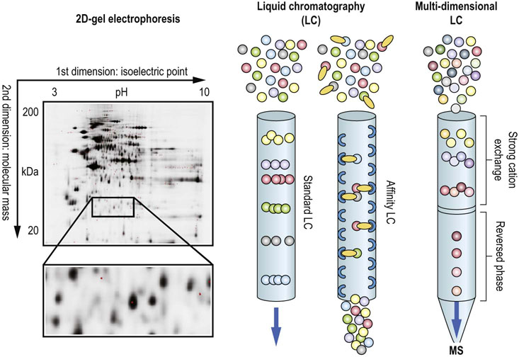
Fig. 36.9 Protein and peptide separation techniques.
The left panel shows a 2D gel where protein lysates were separated by isoelectric focusing in the 1st dimension, and according to molecular weight in the 2nd dimension. Protein spots were visualized with a fluorescent stain. The middle panel illustrates the principles of LC, where proteins or peptides are separated by differential physicochemical interactions with the resin as the flow through the column. A variation is affinity LC, where the resin is modified with an affinity group that retains molecules which selectively bind to these groups. The right panel demonstrates the setup for multi-dimensional LC, where a strong cation exchange column is directly coupled to a reversed-phase column enabling a 2-step separation by hydrophilicity and hydrophobicity. The eluate can be directly infused into a mass spectrometer (MS) for peptide identification.

A classic protein separation method is two-dimensional polyacrylamide gel electrophoresis (2DE, 2D-PAGE)

Proteins are separated by isoelectric focusing according to their electrical charge in the first dimension, and according to their size in the second dimension. Labeling the proteins with fluorescent dyes or using fluorescent stains made the method quantitative, but protein spots have to be picked from the gels individually for subsequent identification by mass spectrometry (MS).

Therefore, 2D-PAGE is now much less frequently used, and has been replaced by liquid chromatography (LC), which can be directly coupled to mass spectrometry (MS). Thus, molecules eluting from the chromatographic column can be measured and identified in real time. As for technical reasons MS-based identification works better with smaller molecules, proteins are digested with proteases (usually trypsin) into small peptides before MS analysis. LC separates proteins or peptides on the basis of different physicochemical properties, most commonly the charge of the molecule or its hydrophobicity, using ion exchange or reversed-phase chromatography, respectively. This is achieved by having chemical groups attached to a particulate resin packed into a column and flowing a solution over this. Molecules will bind to the resin (the stationary phase) with differing affinities. Those with a high affinity will take longer to traverse the length of the column and hence will elute from the column at a later time. Molecules are therefore separated in time in the effluent that elutes off the column. Affinity chromatography uses specialized resins that strongly bind to certain chemical groups or biological epitopes and retain proteins carrying these groups. For instance, resins containing chelated Fe³⁺ or TiO₂ (immobilized metal affinity chromatography, IMAC) bind phosphate and are used to select phosphorylated peptides. LC also can be carried out in two dimensions. Adding a strong cation exchange (SCX) chromatography step before IMAC removes many non-phosphorylated peptides, enhancing the enrichment of phosphosphopeptides in the IMAC step.

The first 2D LC method with direct coupling of the two dimensions is called multidimensional protein identification technology (MudPIT)

In MudPIT the total protein content of the sample is first digested with trypsin, and the resulting peptides are fractionated by an SCX column, which separates peptides according to charge. Then, the peptide fractions are further separated by reversed-phase LC and directly injected into the MS. Modern fast-scanning, high-resolution MS instruments coupled to high-resolution separation LC now make it possible to dispense with the first dimension for all but the most complex samples. This method of MS-enabled, peptide-based protein identification is often referred to as ‘shotgun proteomics’.

Protein identification by mass spectrometry (MS)

Mass spectrometry is a technique used to determine the molecular masses of molecules in a sample

MS can also be used to select an individual component from the mixture, break up its chemical structure and measure the masses of the fragments, which can then be used to determine the structure of the molecule. There are many different types of mass spectrometers available, but the underlying principles of mass spectrometry are relatively simple. The first step in the process is to generate charged molecules, ions, from the molecules in the sample. This is relatively easily achieved for many soluble biomolecules because their polar chemistry provides groups that are easily charged. For example, the addition of a proton (H⁺) to the side-chain groups on the basic amino acids lysine, arginine or histidine gives a positively charged molecule. When a charged molecule is placed in an electric field, it will be repelled by an electrode of like sign and attracted by an electrode of opposite sign, accelerating the molecule towards the electrode of opposite charge. Since the force is equal for all molecules, larger molecules will accelerate less than small molecules (force = mass × acceleration), so small molecules will acquire a higher velocity. This is utilized to determine the mass. For example, after the molecules have been accelerated, the time then taken for them to travel a certain distance can be measured and related to the mass. This is called time-of-flight mass spectrometry.

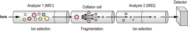
A tandem mass spectrometer is effectively two mass spectrometric analyzers joined together sequentially, with an area between them where molecules can be fragmented

The first analyzer is used to select one of the molecules from a mixture based on its molecular mass, which is then broken up into smaller parts, usually by collision with a small amount of gas in the intermediate region (called the collision cell). The fragments that are generated are then analyzed in the second mass spectrometer (Fig. 36.10). As peptides tend to fragment at the peptide bond, the fragment peaks are separated by the masses of the different amino acids in the corresponding sequence. This result is, in principle, similar to the Sanger method of DNA sequencing, allowing the peptide sequence to be deduced. However, in contrast to Sanger DNA sequencing, peptide fragmentation is not uniform, and the spectra usually only cover part of the sequence, leaving gaps and ambiguous sequence reconstruction. Therefore, the peptide sequence is predicted based on a statistical matching of observed masses against a virtual digest and peptide fragmentation of proteins in a database (Fig. 36.11). With today's highly accurate MS and well-annotated databases, these computational sequence predictions are very reliable. It also demonstrates that proteomics is intimately reliant on the quality and completeness of genome sequencing, and genome databases that are used to infer the encoded proteins.

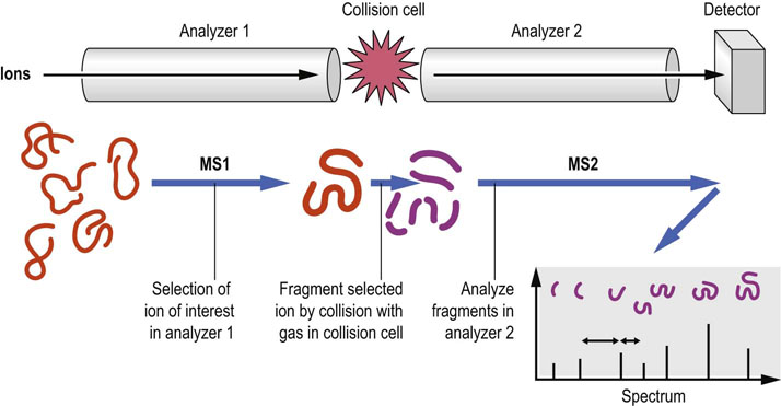
Fig. 36.10 The basic principles of tandem mass spectrometry.
See text for details. MS, mass spectrometer.

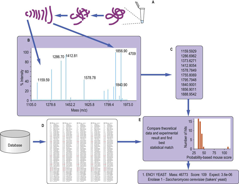
Fig. 36.11 Protein identification by mass spectrometry.
A typical workflow: (A) the sample is digested with a specific protease, usually trypsin, to give a set of smaller peptides which will be unique to the protein; (B) the mass of a subset of the resulting peptides is measured using MS; in tandem MS each peptide is fragmented and the mass of the fragments is measured as well; (C) a list of the observed experimental masses is generated from the mass spectrum; (D) a database of protein sequences is theoretically digested (and fragmented in the case of tandem MS) in silico, and a set of tables of the expected peptides generated; (E) the experimental data are compared to the theoretical digested database and a statistical score of the fit of the experimental to theoretical data is generated, giving a ‘confidence’ score, which indicates the likelihood of correct identification.

MS measures and fragments peptides as they elute from the LC, resulting in abundant proteins being identified many times, whereas low-abundant proteins are overlooked if the MS is overwhelmed by a flow of abundant peptides. This is a main reason why protein or peptide pre-fractionation increases the number of successfully identified proteins. This workflow requires measuring the whole protein complement even when one only is interested in a few specific proteins.

To enable the targeted identification of specific proteins, a technique was developed, called selected reaction monitoring (SRM) or multiple reaction monitoring (MRM)

This method uses MS1 to select a peptide ion out of a mixture, then fragment it and select defined fragment masses for detection in MS2 (Fig. 36.12). A software protocol for MS1 peptide selection and MS2 fragment detection gives unique protein identifications based on the measurement of a few selected peptides. This is a powerful method to streamline the identification of proteins from complex samples by systematically monitoring only the most informative peptide fragmentations. The peptide atlas (www.peptideatlas.org/) is a database of such informative fragments, and will greatly facilitate the systematic analysis of proteomes and sub-proteomes.

Fig. 36.12 The principles of selected reaction monitoring (SRM) or multiple reaction monitoring (MRM) experiments.
See text for details.

Quantitative mass spectrometry

MS can be made quantitative in a number of ways. If possible, samples can be grown in a selective medium that provides an essential amino acid in the natural form (the ‘light’ form) or isotopically labeled with a stable isotope (for example, ¹³C or ²H, the ‘heavy’ form) that makes all of the peptides containing this amino acid appear heavier in the mass spectrometer. This is called the stable isotope labeling with amino acids in cell culture (SILAC) method, and is one of the most widely used and robust of the labeling technologies (Fig. 36.13). The samples are mixed together and analyzed using the shotgun approach. The ratios of ‘heavy’ to the equivalent ‘light’ peptides are used to determine the relative quantities of the protein from which they were derived.

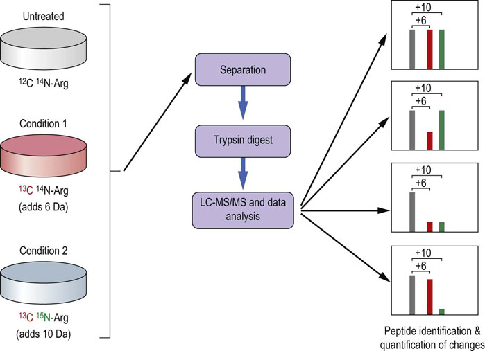
Fig. 36.13 Stable isotope labeling with amino acids in cell culture (SILAC) for quantitative mass spectrometry.
See text for details.

Alternative methods include chemically reacting the proteins in the sample (using, for example, the isotope coded affinity tags, ICAT), or the peptides after digestion of the sample (e.g. in isobaric tags for relative and absolute quantitation, iTRAQ), with a ‘light’ or equivalent isotopically labeled ‘heavy’ chemical reagent, then mixing the samples and analyzing them as for the SILAC approach. Direct comparison of 1D-LC runs based on the normalized signal intensity without the need for labeling is also possible due to improvements in the reproducibility of LC and software. In addition, counting of peptide ions in the mass spectrometer have led to so-called label-free quantitation methods that are rapidly improving and soon may allow accurate quantification without the need to label cells or proteins. The advantage of these methodologies is that the analysis is easily automated and that approaches can be used to get information on proteins that do not work well in the 2DE approach, such as membrane proteins, small proteins and proteins with extreme pIs (e.g. histones). The disadvantage is that information on post-translational modifications is usually lost, and digesting the sample generates a much more complex sample for the separation step.

Non-mass spectrometry based technologies

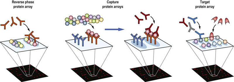
While MS remains a main stay technique used for proteomics, a variety of other methods are becoming established. Protein microarrays are conceptually similar to those used for transcriptomics. They come in three versions (Fig. 36.14). In the reverse phase protein array (RPPA) lysates of cells or tissues are spotted on a microscope slide with a protein-friendly coating. These arrays are then probed with an antibody specific to a protein or a certain PTM. After washing to remove unbound antibodies, successful binding events are visualized by a secondary anti-antibody antibody, which carries a detectable label, usually a fluorescent dye. Thereby, a large number of samples or treatment conditions can be compared simultaneously. The success of this method is completely dependent on the specificity of the antibody, and constrained by the limited availability of high-quality mono-specific antibodies. In the capture array, antibodies are deposited onto the array, which then is incubated with a protein lysate. Detection of the captured proteins is by another antibody. Thus, the overall specificity is the overlap between the specificities of the capturing and detecting antibodies, ameliorating the limitation that each antibody should be absolutely specific. Target arrays contain a single species of purified protein in each spot. These arrays are used to find binding partners for specific proteins. They can be probed with another purified protein, or with a mixture of antibodies, e.g. from patient sera, to determine whether a patient has antibodies against particular proteins. Protein microarrays can be used to quantify the amount of the protein present in a sample and thus lend themselves for clinical diagnostics.

Fig. 36.14 Protein (micro)arrays.
See text for details.

The Human Protein Atlas (HPA) (www.proteinatlas.org/) aims to generate antibodies to every protein in the human proteome, and use these to visualize proteins and their subcellular localization in healthy and diseased human tissues

In 2012 the HPA comprised more than 14,000 proteins, i.e. approximately 70% of gene products, if splice forms and other variants are neglected. Efforts to include protein variants and post-translational modifications are underway. Thus, the HPA is becoming a major resource for proteome analysis.

Microscopy has also become a tool that is frequently used in spatial proteomics, to assess where proteins are localized in the cell and how this changes under different conditions. This has been enabled by the advances in the intracellular expression of proteins that are a fusion between the proteins of interest and green fluorescent protein (GFP) or its analogues. The cellular location of the protein can then be tracked by microscopy by following the fluorescent signal of the protein attached to it. There are now analogues of GFP that emit at a wide range of wavelengths, meaning that three, or even four, proteins can be followed in parallel.

Advanced concept box Nuclear magnetic resonance spectroscopy

Nuclear magnetic resonance (NMR) spectroscopy gives useful structural information on molecules that can be used to identify them. Atomic nuclei behave like small magnets, so when they are put in a strong magnetic field they align with the field. Application of an appropriate energy (radiofrequency electromagnetic radiation) causes the nuclei to flip and align against the field. They then return to their ground state once the irradiation is turned off by flipping back, and as they do so they emit specific frequencies of radiation. These can be recorded and plotted. Each nucleus in a molecule that has a unique environment will emit a unique frequency, and nuclei bonded together or close together in space will interact with adjacent nuclei (coupling), and this can also be measured. This rich information on the molecule allows the structural elements to be determined, and the amplitude of the signals can be used to reasonably accurately quantify the amount of material. This is very useful in metabolomics. The main limitation is that the NMR spectrum quickly becomes congested with information from a complex sample, so high resolution (coming from very strong magnetic fields) is required, and the technique is relatively insensitive, having a limit of detection 3–4 orders of magnitude worse than mass spectrometry.

Metabolomics

Metabolites are the small chemical molecules, such as sugars, amino acids, lipids and nucleotides, present in a biological sample. The study of the metabolite complement of a sample is called metabolomics, while the quantitative measurement of the dynamic changes in the levels of metabolites as a result of a stimulus or other change is often referred to as metabonomics. The words metabolomics and metabonomics are often used interchangeably, although purists will claim that while both involve the multiparametric measurement of metabolites, metabonomics is dedicated to the analysis of dynamic changes of metabolite levels, whereas metabolomics focuses on identifying and quantifying the steady-state levels of intracellular metabolites. Metabolomics is the most commonly used generic term.

Metabolomics gives another level of information on a biological system

It provides information on the results of the activity of enzymes, which may not depend on the abundance of the protein alone, as this may be modulated by supply of substrates, the concentration of cofactors or products, and effect of other small molecules or proteins that modulate the activity of the enzyme (effectors). In some ways, metabolomics may be easier to perform than proteomics. In the metabolome, there is an amplification of any changes that occur in the proteome, as the enzymes will turn over many substrate molecules for each molecule of enzyme. The methods used to look for a metabolite in each organism will be the same, as many of the metabolites will be identical, unlike proteins, whose sequences are much less conserved between organisms. Thus, metabolic networks are more constrained, making them easier to follow.

However, the analysis of the metabolome is still complex as it is very dynamic, many metabolites give rise to a number of molecular species by forming adducts with different counter ions, and xenobiotics, molecules that do not come from the host but from foodstuffs, drugs, the environment or even the microflora in the gut, complicate the analysis greatly; the actual metabolome may be getting close to being as complicated as the proteome.

In a similar way, lipidomics has become a topic in its own right, studying the dynamics changes in lipids in diverse functions such as membranes, lipoproteins, and as signaling molecules. In 2007, the Human Metabolome Project released the first draft of the human metabolome consisting of 2500 metabolites, 3500 food components and 1200 drugs. Currently, there is information on approximately 20,000 metabolites, approximately 1600 drug and drug metabolites, 3100 toxins and environmental pollutants, and around 28,000 food components.

The most commonly used methods for investigating metabolites are mass spectrometry, often coupled to LC, as used in proteomics, and nuclear magnetic resonance (NMR) spectroscopy. Identification of signals corresponding to specific metabolites can then be used to quantify these metabolites in a complex sample, and see how they change.

Metabolomics can be broken down into a number of areas

Metabolic fingerprinting: taking a ‘snapshot’ of the metabolome of a system, generating a set of values for the intensity of a signal from a species, without necessarily knowing what that species is. Often there is no chromatographic separation of species. It is used for biomarker discovery.

Metabolite profiling: generating a set of quantitative data on a number of metabolites, usually of known identity, over a range of conditions or times. It is used for metabolomics, metabonomics, and systems biology and biomarker discovery.

Metabolite target analysis: measuring of the concentration of a specific metabolite or small set of metabolites over a range of conditions or times.

Biomarkers

Biomarkers are markers that can be used in medicine for the early detection, diagnosis, staging or prognosis of disease, or for determination of the most effective therapy

A biomarker is generally defined as a marker that is specific for a particular state of a biological system. The markers may be metabolites, peptides, proteins or any other biological molecule, or measurements of physical properties, e.g. blood pressure. The importance of biomarkers is rapidly increasing because the trend to personalized medicine will be impossible to sustain without a detailed and objective characterization of the patients afforded by biomarkers. Biomarkers can arise from the disease process itself or from the reaction of the body to the disease. Thus, they can be found in body fluids and tissues. For ease of sample sourcing and patient compliance, most biomarker studies use urine or plasma, although saliva, interstitial fluid, nipple duct aspirates, and cerebrospinal fluid also have been used.

The most common methods for biomarker discovery have developed from those used in transcriptomics, proteomics and metabolomics, i.e. gene arrays, mass spectrometry, often coupled to chromatography, and NMR spectroscopy

Biomarker discovery is often done on small patient cohorts but, to be clinically useful, a robust statistical analysis of a large number of samples from healthy and sick individuals in well-controlled studies is required. Improvements in methods for statistical analysis, coupled to detection methods that can differentiate hundreds to tens of thousands of individual components in the complex sample, have improved the selectivity to the level where these aims are achievable. It is usually necessary to define a number of markers, i.e. a biomarker panel, that are indicative for a given disease in order to achieve selectivity rather than just detecting a general systemic response such as the inflammatory response or a closely related disease. In theory, it is not necessary to actually identify what the biomarker is, although doing so may give insight into the underlying biochemistry of the disease, and many regulatory authorities demand that the markers are identified before a method can be licensed. It may also allow subsequent development of cheaper and higher throughput assays.

Some well-known examples of biomarkers are the measurement of blood glucose levels in diabetes, prostate-specific antigen for prostate cancer, and HER-2 or BRCA1/2 genes in breast cancer

Biomarker research can also elucidate disease mechanisms and further markers or potential drug targets. For example, using a 2DE approach to determine which DNA repair pathways had been lost in breast cancer led to the discovery that cancers deficient in the BRCA1/2 genes are sensitive to the inhibition of another DNA repair protein, poly(ADP-ribose) polymerase 1, known as PARP-1. Inhibitors of PARP-1 are showing promise in clinical trials for the treatment of BRCA1/2 deficient tumors.

Data analysis and interpretation by bioinformatics and systems biology

The -omics experiments can generate many gigabytes, and even terabytes of information. However, data are not information, and information is not knowledge. Making use of this data is fundamentally dependent on computational methods. Bioinformatics is the term used for computational methods for the extraction of useful information from the complex datasets generated from-omics experiments: for instance, generating quantitative data on gene transcription from next-generation sequencing, or identifying proteins from the fragments generated in mass spectrometry. The annotation of these datasets, for instance with protein function or localization, and the hierarchical organization of the data, can be seen as static information. Systems biology takes this further and generates computational and mathematical models from our knowledge of biology and the refined data coming from bioinformatics analysis. These models are used to simulate biochemical and biological processes in silico (an expression meaning ‘performed on computers’) and reveal how complex systems, such as intracellular signaling networks, actually work.

Summary

The -omics approaches hold a huge potential for the risk assessment, early detection, diagnosis, stratification and tailored treatment of human diseases.

The -omics technologies are being introduced into clinical practice, with genomics and transcriptomics leading the way. This is mainly because DNA and RNA have defined physicochemical properties that are amenable for amplification, and the design of robust assay platforms compatible with the routines of clinical laboratories. For instance, PCR and DNA sequencing are used in forensic medicine to establish paternity and to determine the identity of DNA samples left at crime scenes. Genetic tests for the diagnosis of gene mutations and inherited diseases are now in place.

Transcriptomic-based microarray tests for breast cancer have been approved, and similar tests for other diseases are becoming available.

Proteomics and metabolomics require specialist equipment and expertise, which are difficult to put into the routine clinical laboratory. However, their information content exceeds that of genomics and with further progress in technology, their clinical applications will become reality.

The benefits of -omics technologies are obvious, mainly in risk assessment and the design of personalized treatments. However, there are also huge ethical implications pertaining to the use of this information, and new regulatory guidelines will be needed.

Active learning

1. Why does the information increase when moving from studying genes to studying proteins?

2. What is a gene and how is gene transcription regulated?

3. How can we study gene mutations?

4. How can we determine the sequence of DNA and proteins?