Physical Principles of Computed Tomography
The information presented in a computed tomography (CT) image differs from a conventional radiographic image in several respects. The most obvious is that CT shows cross-sectional (transaxial) views of patient anatomy. In addition, CT shows three-dimensional (3D) images that are computer generated (digital image after processing) with use of the transaxial data set (Fig. 4-1). Other significant differences in CT imaging will become apparent in the following chapters. In this presentation of the physical principles of CT, a review of conventional tomography and the limitations of radiography is helpful to understand the CT image.
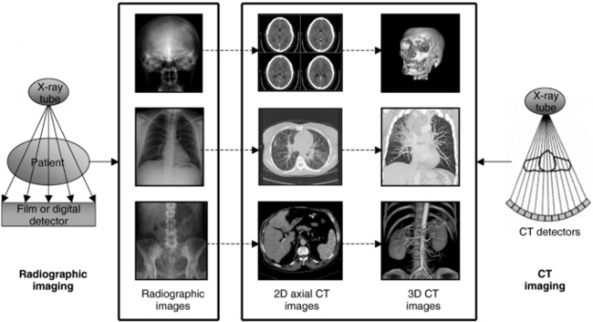
FIGURE 4-1 The most conspicuous difference between conventional radiographic imaging and CT imaging is that CT shows cross-sectional or transaxial anatomy, that can be subject to digital postprocessing operations to produce 3D images. 3D CT images courtesy Philips Medical Systems.
LIMITATIONS OF RADIOGRAPHY AND TOMOGRAPHY
In both radiography and tomography, x rays pass through the patient and are absorbed in different ways by the body’s tissues. For example, because bone is denser, it absorbs more x rays than do the less-dense soft tissues. This differential absorption is contained in the x-ray beam that passes through the patient and is recorded on radiographic film or a radiographic digital detector, such as a computed radiography imaging plate, for example.
Limitations of Film-Based Radiography
The major shortcoming of radiography is the superimposition of all structures on the film, which makes it difficult and sometimes impossible to distinguish a particular detail (Fig. 4-2). This is especially true when structures differ only slightly in density, as is often the case with some tumors and their surrounding tissues. Although multiple views such as laterals and obliques can be taken to localize a structure, the problem of superimposition in radiography still persists.
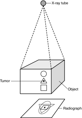
FIGURE 4-2 The major shortcoming of radiography is that the superimposition of all structures on the radiograph makes it difficult to discriminate whether the tumor is in the circle, triangle, or square. From Seeram E: Computed tomography technology, Philadelphia, 1982, WB Saunders.
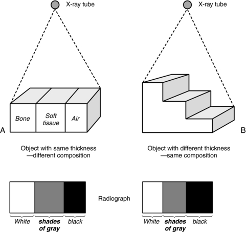
A second limitation is that radiography is a qualitative rather than quantitative process (Fig. 4-3). It is difficult to distinguish between a homogeneous object of nonuniform thickness and a heterogeneous object (Fig. 4-3 includes bone, soft tissue, and air) of uniform thickness (Marshall, 1976).
Limitations of Conventional Tomography
The problem of superimposition in radiography can be somewhat overcome by conventional tomography (Bocage, 1974; Vallebona, 1931). The most common method of conventional tomography is sometimes referred to as geometric tomography to distinguish it from CT (Fig. 4-4). When the x-ray tube and film are moved simultaneously in opposite directions, unwanted sections can be blurred while the desired layer or section is kept in focus.
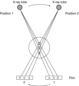
FIGURE 4-4 Basic principles of conventional tomography. The x-ray tube and film move simultaneously and in opposite directions to ensure that the desired section ( ) of the patient is imaged by blurring out structures above (
 ) and below (
 ) the plane of interest (). From Seeram E: Computed tomography technology, Philadelphia, 1982, WB Saunders.
The immediate goal of tomography is to eliminate structures above and below the focused section, or the focal plane. However, this is difficult to achieve, and under no circumstances can all unwanted planes be removed. The limitations of tomography include persistent image blurring that cannot be completely removed, degradation of image contrast because of the presence of scattered radiation created by the open geometry of the x-ray beam, and other problems resulting from film-screen combinations.
In addition, both radiography and tomography fail to adequately demonstrate slight differences in subject contrast, which are characteristic of soft tissue. The differences for soft tissues such as human fat, water, human cerebrospinal fluid, human plasma, monkey pancreas, monkey white matter, monkey gray matter, monkey liver, monkey muscle, and human red blood cells are 0.194, 0.222, 0.227, 0.227, 0.230, 0.230, 0.235, 0.236, 0.238, and 0.246, respectively (Ter-Pogossian et al, 1974). Radiographic film is not sensitive enough to resolve these small differences because typical film-screen combinations used today can only discriminate x-ray intensity differences of 5% to 10%.
The limitations of radiography and tomography result in the inability of film to image very small differences in tissue contrast. In addition, contrast cannot be adjusted after it has been recorded on the film. Digital imaging modalities such as CT, for example, can alter the contrast to suit the needs of the human observer (radiologists and technologists) by use of various digital image postprocessing techniques (see Chapter 3).
Enter CT
The goal of CT is to overcome the limitations of radiography and tomography by achieving the following (Hounsfield, 1973):
The basic methodological approach to these three tasks is shown in Figure 4-5. A few important points can be noted from this figure, as follows:
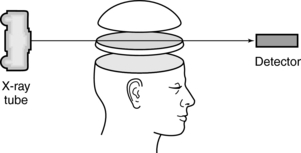
FIGURE 4-5 In CT a thin beam is transmitted through a specific cross-section, striking special detectors opposite the x-ray tube.
1. A beam of x rays is transmitted through a specific cross-section of the patient. This procedure removes the problem of superimposition of structures above and below the specific cross-section or slice of tissue.
2. The beam of x rays is highly collimated into a thin beam (a very narrow beam) that only passes through the cross-section of tissue to be imaged. This procedure is intended to minimize scatter production and therefore improve the contrast of the image.
3. When the x-ray beam passes through the patient, it strikes special electronic detectors positioned opposite the x-ray tube. These detectors are quantitative and can measure very small differences in tissue contrast. (However, the film-screen detector in radiography is considered a qualitative detector and cannot record these small differences.) In addition, the analog signals from the electronic detectors are first converted into digital data and are subsequently processed by a digital computer that uses special algorithms to reconstruct an image of the cross-section.
PHYSICAL PRINCIPLES
CT can be described in terms of physical principles and technological considerations. The physical principles involve physics and mathematical concepts to understand the way the image is produced, and the technological considerations involve the practical implementation of scientific and engineering principles such as computer science and technology. The physical principles and technology of CT include the three processes referred to in Chapter 1: data acquisition, data processing, and image display, storage, and communication. This section discusses each process in basic terms; they are described in more detail in later chapters.
Data Acquisition
Data acquisition refers to the systematic collection of information from the patient to produce the CT image. The two methods of data acquisition are slice-by-slice data acquisition and volume data acquisition (Fig. 4-6).
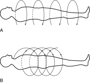
In conventional slice-by-slice data acquisition, data are collected through different beam geometries to scan the patient. Essentially, the x-ray tube rotates around the patient and collects data from the first slice. The tube stops, and the patient moves into position to scan the next slice. This process continues until all slices have been individually scanned.
In volume data acquisition, a special beam geometry referred to as spiral or helical geometry is used to scan a volume of tissue rather than one slice at a time (see Fig. 4-6). In spiral/helical CT, the x-ray tube rotates around the patient and traces a spiral/helical path to scan an entire volume of tissue while the patient holds a single breath. This method generates a single slice per one revolution of the x-ray tube and is often referred to as a single-slice spiral/helical CT (SSCT). To improve the volume coverage speed performance of SSCT, multislice spiral/helical CT (MSCT) has become available for faster imaging of patients. MSCT scanners generate multiple slices per one revolution of the x-ray tube. For example, MSCT scanners can now generate 4, 8, 16, 32, 40, or 64 slices per revolution of the x-ray tube. The most recent MSCT scanner commercially available for clinical imaging of patients (at the time of writing this chapter) is the 64-slice MSCT scanner. Additionally, in 2007, an MSCT scanner that can produce 320 slices per revolution of the x-ray tube became commercially available.
The first step in data acquisition is scanning (Fig. 4-7). During scanning, the x-ray tube and detectors rotate around the patient to collect views (intensity readings). The detectors measure the radiation transmitted through the patient from various locations. As a result, relative transmission values (Hounsfield, 1973) or attenuation measurements (Sprawls, 1995) can be calculated as follows:
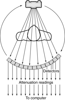
FIGURE 4-7 During scanning, the x-ray tube and detectors rotate around the patient to collect views.

The relative transmission values are sent to the computer and stored as raw data.
A large number of transmission measurements are needed to reconstruct the CT image. In general, several hundred views are obtained. Each view is composed of a number of rays, and the total transmission measurements for each scan is given by the following relationship (Sprawls, 1995):
Radiation Attenuation: The problem in CT is to determine the attenuation in the tissues and use this information to reconstruct an image of the slice of tissue. The solution to this problem is complex and involves physics, mathematics, and computer science. This book takes a fundamental approach to the problem and its solution. The study begins with an understanding of attenuation of radiation in general and attenuation in CT in particular.
Attenuation is the reduction of the intensity of a beam of radiation as it passes through an object—some photons are absorbed, but others are scattered. Attenuation depends on the electrons per gram, atomic number, tissue density, and radiation energy used. In addition, because there are two types of radiation beams (homogeneous and heterogeneous), a study of how each of these beams is attenuated is important to understand the problem in CT. Attenuation in CT depends on the effective atomic density (atoms/volume), the atomic number (Z) of the absorber, and the photon energy.
In a homogeneous beam, all the photons have the same energy, whereas in a heterogeneous beam the photons have different energies. A homogeneous beam is also referred to as a monochromatic or monoenergetic beam, and a heterogeneous beam is referred to as a polychromatic beam.
When Hounsfield invented the CT scanner, he used a homogeneous beam (Fig. 4-8) in his initial experiments because such a beam satisfies the requirements of the Lambert-Beer law, an exponential relationship that describes what happens to the photons as they travel through the tissues according to the following attenuation:
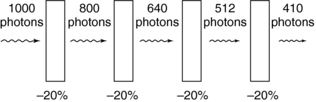
FIGURE 4-8 Attenuation of a homogeneous beam of radiation through water. The absorber is 1 cm of water.

where I is the transmitted intensity, I0 is the original intensity, x is the thickness of the object, e is Euler’s constant (2.718), and μ is the linear attenuation coefficient.
The goal of CT is to calculate the linear attenuation coefficient μ, which indicates the amount of attenuation that has occurred. Therefore it is a quantitative measurement with a unit of per centimeter (cm−1)—hence the term linear (Bushong, 2004; Kalender, 2005).
The equation I = I0e–μx can be solved to find the value of μ:
where ln is the natural logarithm. In CT, the values of I and I0 are known (these are measured by the detectors), and x is also known. Hence μ can be calculated.
Figure 4-8 shows the attenuation of a homogeneous beam of radiation. Each section of the absorber attenuates the beam by equal amounts; that is, each 1-cm section removes 20% of the photons remaining in the beam. The initial beam intensity of 1000 photons is reduced to 410 photons. In other words, the quantity of photons is reduced. In a homogeneous beam the quality of the beam, or beam energy, does not change. If the starting beam energy is 88 kiloelectron volts (keV), the transmitted photons all have an energy of 88 keV.
In the early experiments conducted by Hounsfield, the radiation was from a gamma source and the attenuation was that of a homogeneous beam. One problem he encountered was that it took too long to scan and produce an image, and therefore he substituted a beam produced by a conventional x-ray tube. This beam is a heterogeneous beam of radiation that consists of a range of energies. The attenuation of a heterogeneous or polychromatic beam is somewhat different from that of a homogeneous beam, and therefore Hounsfield had to make several assumptions and adjustments to determine the linear attenuation coefficients.
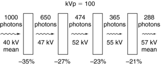
During the attenuation of a heterogeneous beam (Fig. 4-9), as the beam passes through equal thicknesses of material, the attenuation is not exponential but rather both the quantity and quality of the photons change. In Figure 4-9, the initial quantity of photons is 1000 with a mean beam quality (energy) of 40 kilovolts (kV). Each block of water removes different quantities of photons, and the mean energy of the transmitted photons increases to 57 kV. The first centimeter of water attenuates more photons than subsequent 1-cm blocks of water. Also, the lower-energy photons are absorbed, which allows the higher-energy photons to pass through. As a result, the penetrating power of the photons increases and the beam becomes harder.
The equation I = I0e–μx applies only to a homogeneous beam. It then follows that in CT, which is based on the use of a heterogeneous beam, it is necessary to make the heterogeneous beam approximate a homogeneous beam to satisfy the equation.
It was stated earlier that attenuation is the result of absorption and scattering. X rays can be attenuated because of the photoelectric effect, or they can be attenuated and scattered by the Compton effect. The total attenuation is then given by
where μp is the linear attenuation coefficient that results from photoelectric absorption, and μc is the linear attenuation coefficient that results from the Compton effect.
The photoelectric effect occurs mainly in tissues with a high atomic number, Z (such as bone, contrast medium) and occurs minimally in some soft tissues and substances with a lower Z. The Compton effect occurs in soft tissues, and differences in density result in differences in Compton interactions. In addition, the photoelectric effect depends on the beam energy (kilovolts); however, the Compton effect is less likely to dominate as the beam energy increases and “the energy dependence is not nearly as dramatic as it is with the photoelectric effect” (Morgan, 1983).
Equation 4-2, like Equation 4-1, holds true only for a homogeneous beam of radiation. Because a heterogeneous beam is used in CT, how is the linear attenuation coefficient determined in CT? The concern is with the number of photons, N, that pass through the tissue during scanning, rather than with the intensity, I. Equation 4-1 can therefore be expressed as
where N is the number of transmitted photons, N0 is the number of photons entering the tissue (incident photons), x is the thickness of the tissue, μ is μp + μc (linear attenuation coefficients of the tissue), and e is the base of the natural logarithm.
Equation 4-3 applies to a homogenous block of tissue. However, a slice of tissue in the patient through which the radiation passes is not homogeneous because the tissue is composed of several different substances. In this case, the slice is divided into a number of small regions, “each characterized by its own linear attenuation coefficient” (Morgan, 1983). This can be shown as

In this situation, the linear attenuation coefficients can be determined as follows:

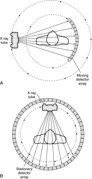
Data Acquisition Geometries: The way that the x-ray tube and detectors are arranged to collect transmission measurements describes the data acquisition geometry of the CT system. Two types of geometries are illustrated in Figure 4-10. In Figure 4-10, A, the x-ray tube and detectors are coupled and rotated 360 degrees around the patient to collect transmission measurements by using a fan beam of radiation. In Figure 4-10, B, the x-ray tube rotates 360 degrees around the patient and is positioned inside a stationary ring of detectors. The radiation beam also describes a fan. It is interesting to note that the geometry shown in Figure 4-10, A, has become commonplace in modern CT scanners.
Data Processing
Data processing essentially constitutes the mathematical principles involved in CT. Data processing is basically a two-step process (Fig. 4-11). First, the raw data (data received from the detectors) undergo some form of preprocessing, in which corrections are made and some reformatting of the data occurs. This is necessary to facilitate the next step in data processing, image reconstruction. In this step, the scan data, which represent attenuation readings, are converted into a digital image characterized by CT numbers (Fig. 4-12).
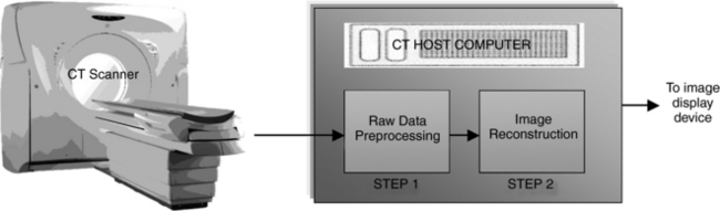
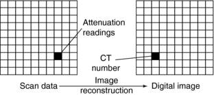
FIGURE 4-12 Data acquired by scanning an object measures beam penetration. A digital image is created by converting these data into CT numbers.
Conversion of the attenuation readings into a CT image is accomplished by mathematical procedures referred to as reconstruction algorithms. These algorithms include simple back-projection, iterative methods, and analytic methods. For MSCT scanners that offer 16 and 64 slices per revolution of the x-ray tube, other reconstruction algorithms referred to as cone-beam algorithms are used (Kalender, 2005). These algorithms are described further in Chapter 6. After data processing, the reconstructed image is displayed for viewing and subsequently sent for storage or communicated through the picture archiving and communication system (PACS) to remote sites for review by other physicians (Fig. 4-13).
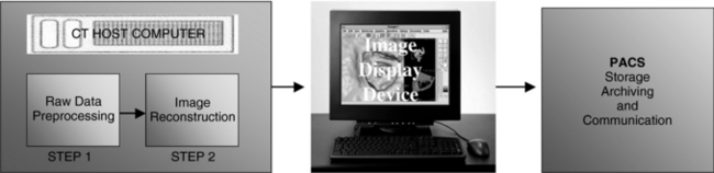
FIGURE 4-13 The reconstructed CT image is displayed for viewing and subsequently sent for storage or communicated by the PACS to physicians at remote sites.
CT Numbers: As shown in Figure 4-12, each pixel in the reconstructed image is assigned a CT number. CT numbers are related to the linear attenuation coefficients (μ) of the tissues that comprise the slice (Table 4-1) and can be calculated as follows:
TABLE 4-1
Linear Attenuation Coefficients for Various Body Tissues*
| Tissues | Linear Attenuation Coefficient (cm−1) |
| Bone | 0.528 |
| Blood | 0.208 |
| Gray matter | 0.212 |
| White matter | 0.213 |
| Cerebrospinal fluid | 0.207 |
| Water | 0.206 |
| Fat | 0.185 |
| Air | 0.0004 |
where μt is the attenuation coefficient of the measured tissue, μw is the attenuation coefficient of water, and K is a constant or contrast factor.
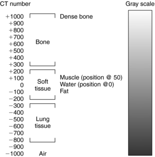
The value of K determines the contrast factor, or scaling factor. In the first EMI scanner, the value of K was 500, which resulted in a contrast scale of 0.2% per CT number. The CT numbers obtained with a contrast factor of 500 were referred to as EMI numbers. Later, the contrast factor was doubled to give a factor of 1000, and the CT numbers obtained with this factor are referred to as the Hounsfield (H) scale. The H scale expresses μ more precisely because the contrast scale is now 0.1% per CT number. (Both the H and EMI scales are shown in Fig. 4-14.) CT numbers are established on a relative basis with the attenuation of water as a reference. Thus the CT number for water is always 0, whereas those for bone and air are +1000 and –1000, respectively, on the H scale. An elaboration of the H scale for several tissues is illustrated in Figure 4-15. Note the range of CT numbers for water, air, fat, kidney, pancreas, blood, and liver.

FIGURE 4-14 Distribution of CT numbers on the Hounsfield and EMI scales. From Seeram E: Computed tomography technology, Philadelphia, 2001, WB Saunders.
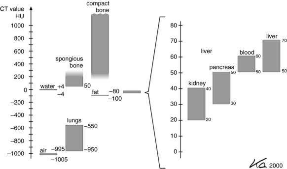
FIGURE 4-15 An elaboration of the Hounsfield scale for several tissues not shown in Figure 4-14. From Kalender WA: Computed tomography, ed 2, Erlangen, Germany, 2005, Publicis Kommunikations Agentur Gmbh; © 2005 by Publicis Kommunikations Agentur GmbH, GWA, Erlangen, Germany. Reproduced by permission.
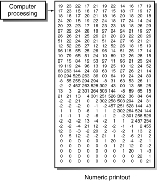
The computer calculates the CT numbers, which can be printed as a numerical image (Fig. 4-16). This image must be converted into a gray-scale image because it is more useful to the radiologist than is a numerical printout. To facilitate this conversion, brightness levels that correspond with the CT numbers must be established (Fig. 4-17). In Figure 4-17, the upper +1000) and lower –1000) limits of the scale represent white and black, respectively. All other values represent various shades of gray.
CT and Energy Dependence: The linear attenuation coefficient (μ) is affected by several factors, including the energy of the radiation. For example, the linear attenuation coefficients for water at 60, 84, and 122 keV are 0.206, 0.180, and 0.166, respectively. It then follows that photon energy also affects CT numbers because they can be calculated on the basis of the attenuation coefficients by the equation
In this summation equation, E represents the photon energy and demonstrates that the attenuation coefficient changes with the beam energy.
In the original CT scanner, CT numbers were calculated on the basis of 73 keV, which is the effective energy of a 230 peak kilovolt beam after passing through 27 cm of water (Zatz, 1981). At 73 keV, the linear attenuation coefficient for water is 0.19 cm–1. For example, if the linear attenuation coefficients for bone and water are 0.38 and 0.19 cm–1, respectively, and the scaling factor (K) of the scanner is 1000, the CT numbers for bone and water can be calculated:
Thus the CT number for bone is 1000.
Thus the CT number for water is 0.
In CT, a high-kilovolt technique (about 120 kV) is generally used for the following reasons:
1. To reduce the dependence of attenuation coefficients on photon energy
These reasons are important to ensure optimum detector response (e.g., to reduce artifacts caused by changes in skull thickness, which can conceal small changes in attenuation in soft tissues and to minimize artifacts resulting from beam-hardening effects).
CT numbers may vary because of their energy dependence. It is therefore essential that the CT system ensure the accuracy and reliability of these numbers because the consequences can be disastrous and might lead to a misdiagnosis. The system incorporates a number of correction schemes to maintain the precision of the CT numbers.
Image Display, Storage, and Communication: The third and final step in the CT process involves image display, storage, and communication. After the CT image has been reconstructed, it exits the computer in digital form (see Figs. 4-12 and 4-16). This must be converted to a form that is suitable for viewing and meaningful to the observer (Seeram, 1982).
Display Device: The gray-scale image is displayed on a television monitor (Cathode ray tube [CRT]) or liquid crystal display, which is an essential component of the control or viewing console (see Fig. 4-13). In the display and manipulation of gray-scale images for diagnosis, it is important to optimize image fidelity (i.e., the faithfulness with which the device can display the image). This is influenced by physical characteristics such as luminance, resolution, noise, and dynamic range. These topics are beyond the scope of this chapter.
Resolution, however, is an important physical parameter of the gray-scale display monitor and is related to the size of the pixel matrix, or matrix size. The display matrix can range from 64 × 64 to 1024 × 1024, but high-performance monitors can display an image with a 2048 × 2048 matrix (Dwyer, et al, 1992).
Windowing: The CT image is composed of a range of CT numbers (e.g., +1000 to –1000, for a total of 2000 numbers) that represent varying shades of gray (see Fig. 4-17). The range of numbers is referred to as the window width (WW), and the center of the range is the window level (WL) or window center (C). Both the WW and WL are located on the control console. These controls can alter the image contrast and brightness. With a WW of 2000 and a WL of 0, the entire gray scale is displayed and the ability of the observer to perceive small differences in soft tissue attenuation will be lost because the human eye can perceive only about 40 shades of gray (Castleman, 1994).
The process of changing the CT image gray scale in this way is referred to as windowing (Fig. 4-18). Although the WW controls the image contrast, the WL or C controls the image brightness. As can be seen in Figure 4-18, as the WL or C increases the image goes from white (bright) to dark (less bright); and the image contrast changes for different values of WWs. The image contrast is optimized for the anatomy under study, and therefore specified values of WW and WL or C must be used during the initial scanning of the patient. Note that in Figure 4-18 three windows are shown: the bone window (optimized for imaging bone), the mediastinal window (optimized for imaging the mediastinal structures), and the lung window (optimized for imaging the lungs). Windowing is described in detail in a later chapter.
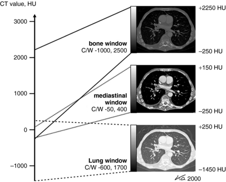
FIGURE 4-18 Windowing is a digital image postprocessing operation intended to alter the image contrast (a function of the WW) and the image brightness (a function of the window center, C, or WL, as it is often referred to). From Kalender WA: Computed tomography, ed 2, Erlangen, Germany, 2005, Publicis Kommunikations Agentur GmbH; 2005 by Publicis Kommunikations Agentur GmbH, GWA, Erlangen, Germany. Reproduced by permission.
Format of the CT Image
The original clinical CT images were composed of an 80 × 80 matrix for a total of 6400 pixels.
The size of the matrix is chosen by the technologist before the CT examination and depends on the anatomy under study. The technologist must select the field of view (FOV) or reconstruction circle, which is a circular region from which the transmission measurements are recorded during scanning. This region is specifically referred to as the scan FOV.
During data collection and image reconstruction, a matrix is placed over the scan FOV to cover the slice to be imaged. In general, a technologist can select the FOV appropriate to the examination within three to four scan FOVs.
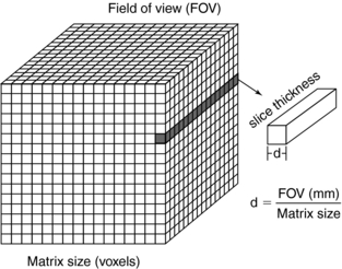
Because the slice to be scanned has the dimension of depth, the pixel is transformed into a voxel, or volume element. The radiation beam passes through each voxel and a CT number is then generated for each pixel in the displayed image. The display FOV can be equal to or less than the scan FOV.
The pixel size can be computed from the FOV and the matrix size through the following relationship:

For example, if the reconstruction circle (FOV) is 25 cm and the matrix size is 5122, the pixel size can be determined as follows:
The pixel size generally ranges from 1 to 10 mm on most scanners. Thus voxel size depends not only on the thickness of the slice but also on the matrix size and the FOV (Fig. 4-19). When the voxel dimensions of length, width, and height are equal, that is, describe a perfect cube, the imaging process is referred to as isotropic imaging (see Chapters 1 and 12).
Finally, each pixel in the CT image can have a range of gray shades. The image can have 256 (28), 512 (29), 1024 (210), or 2048 (211) different gray-scale values. Because these numbers are represented as bits, a CT image can be characterized by the number of bits per pixel. CT images can have 8, 9, 10, 11, or 12 bits per pixel. The image therefore consists of a series of bit planes referred to the bit depth (Fig. 4-20) (Seibert, 1995). The numerical value of the pixel represents the brightness of the image at that pixel position. A 12-bits-per-pixel CT image would represent numbers ranging from –1000 to 3095 for a total of 4096 (212) different shades of gray (Barnes and Lakshminarayanan, 1989).
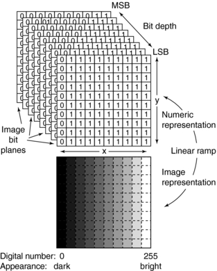
FIGURE 4-20 Representation of the digital image as a stack of bit planes. Encoding of the least significant bit (LSB) to the most significant bit (MSB) as bit planes is shown. The corresponding gray-scale image indicates digital value and brightness relationships. From Seibert JA: Digital image processing basics. In Balter S, Shope TB, editors: RSNA categorical course in physics: physical and technical aspects of angiography and interventional radiology, Oak Brook, Ill, 1995, RSNA.
TECHNOLOGICAL CONSIDERATIONS
The ultimate goal of a CT scanner is to produce high-quality CT images with minimal radiation dose and physical discomfort to the patient. Whether this is achieved depends on the design of the CT system, which influences the performance of the system’s components. In this section, design refers to the technology necessary to produce a CT image.
The technology of a CT scanner encompasses a number of subsystems (Fig. 4-21). The major subsystems are described briefly to demonstrate the flow of data through the system.
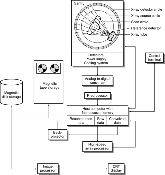
FIGURE 4-21 Fourth-generation CT scanner configuration with major subsystems. From Huang HK: PACS and imaging informatics, Englewood Cliffs, NJ, 2004, John Wiley.
Data Flow in a CT Scanner
The subsystems shown in Fig. 4-21 include the x-ray tube, power supply, and cooling system; beam geometry, defined by collimators and characterized by tube scanning motion; detectors, detector electronics, preprocessors, host computer with fast-access memory, high-speed array processors, digital image processor, storage, display, and system control.
The flow of data from Figure 4-21 is summarized in Figure 4-22. The language that describes some of the events (e.g., convolution and back-projection) is explained further in subsequent chapters.
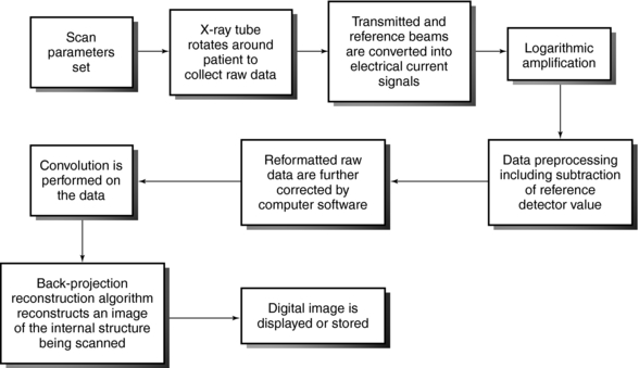
Sequence of Events
The events represented in the data flow are as follows:
1. The x-ray tube (and detectors) rotate around the patient, who is positioned in the gantry aperture for the CT examination. This step is characterized by the beam geometry and method of scanning and involves the passage of x-rays through the patient. The x-ray beam is highly collimated by prepatient collimators.
2. The radiation is attenuated as it passes through the patient. The transmitted photons are measured by two sets of detectors, a reference detector, which measures the intensity of radiation from the x-ray tube, and another set that records x-ray transmission through the patient.
3. The transmitted beam and reference beam are both converted into electrical current signals that are amplified by special circuits. This is followed by logarithmic amplification, in which the relative transmission readings (I0/I) are changed into attenuation (μ) and thickness (x) data through the use of Equation 4-2:
4. Before the data are sent to the computer, they must be converted into digital form. This is done by the analog-to-digital converters, or digitizers. Steps 2, 3, and 4 constitute the second step in the data acquisition process.
5. Data processing begins. The digital data undergo some form of preprocessing, which includes corrections and reformatting. “Some of the corrections to the data will include subtraction of the air reference detector signal to normalize the attenuation data, obtaining local averages of detectors to determine if any detectors are outside a predetermined standard deviation which help locate bad detectors, and corrections due to dead time losses (i.e., detection response time losses) by the individual detectors” (Huang, 2004). The data are now referred to as reformatted raw data. Additional data corrections are performed on the data by using computer software.
6. As shown in Figure 4-22, convolution is performed on the data by the array processors.
7. The specific reconstruction algorithm then reconstructs an image of the internal anatomic structures under examination.
8. The reconstructed image can then be displayed or stored on magnetic or optical tape or disks.
9. The image processor shown in Figure 4-21 allows the performance of various digital image postprocessing operations on the displayed image (Seeram and Seeram, 2008). Figure 4-21 does not show the digital-to-analog converter, a component positioned between the image processor and the CRT display or between the host computer and control terminal, which has a CRT display unit.
10. The control terminal is usually an operator’s control console, which completely controls the CT system.
ADVANTAGES AND LIMITATIONS OF CT
The main advantages of CT stem from the fact that the technique overcomes the limitations of radiography and conventional tomography. Compared with radiography and conventional tomography, CT offers the following advantages:
1. Excellent low-contrast resolution is possible because (1) a highly collimated beam is used to take an image of a cross-sectional slice of the patient and (2) more sensitive radiation detectors (compared with film-screen or digital radiography detectors) are used to measure the radiation transmitted through the slice. CT offers the best low contrast resolution compared with radiography, nuclear medicine, and ultrasonography. For example, the contrast resolution (in millimeters at 0.5% difference) for CT is 4 compared to 10, 10, and 20 for radiography, ultrasonography, and nuclear medicine, respectively. It is interesting to note here that the contrast resolution (mm at 0.5% difference) for magnetic resonance imaging (MRI) is 1 (Bushong, 2003).
2. By changing the WW and WL settings in image windowing, the contrast scale of the image can be varied to suit the needs of the observer (Seeram, 2004; Seeram and Seeram, 2008).
3. With spiral/helical volume data acquisition, CT scanning in spiral/helical geometry has overcome several limitations of conventional start-stop acquisition. Its advantages include volume data acquisition in a single breath rather than slice-by-slice acquisition, improvements in 3D imaging, multiplanar image reformatting, and other applications, such as continuous imaging, CT angiography, and virtual reality imaging, or CT endoscopy.
4. CT has made available a variety of techniques intended to facilitate the diagnostic process such as xenon CT (the use of inhaled stable xenon to study blood flow), quantitative CT (determination of bone mineral content), dynamic CT (rapid-sequence CT scanning to study physiology), perfusion CT, and high spatial resolution CT scanning to optimize the spatial resolution. In addition, CT can assist in radiation treatment planning. Additionally, CT can be coupled to single-photon emission CT (SPECT) and positron emission tomography (PET) scanners to produce fused SPECT/CT and PET/CT images, in an effort to provide more information about the patient’s medical condition.
5. With regard to image manipulation and analysis, the digital nature of the CT image makes it a candidate for digital image processing. Through the application of certain image processing algorithms, the image can be modified to enhance its information content or analyzed to obtain information about the shape and texture of lesions.
6. 3D imaging: CT now produces 3D images routinely. These images are intended to enhance image information content and improve the diagnostic interpretation skills of the radiologist. 3D imaging is described in detail in Chapter 14.
Limitations
CT is not without its limitations. Compared with radiography and tomography, the following disadvantages can be noted:
1. The spatial resolution (line pairs per millimeter) of CT is “notably poorer” (Hendee and Ritenour, 1992) compared with radiography. For example the spatial resolution for CT is 2. For nuclear medicine, ultrasonography, and MRI, the spatial resolution is 0.1, 0.25, and 2, respectively (Bushong, 2003).
2. The dose in CT is generally higher for similar anatomical regions.
3. In CT, it is difficult to image anatomic regions in which soft tissues are surrounded by large amounts of bone, such as the posterior fossa, spinal cord, pituitary, and the interpetrous space (Oldendorf and Oldendorf, 1991). The imaging process may create artifacts that may obscure diagnosis.
4. The presence of metallic objects on the patient produces streak artifacts on CT images. CT also creates other artifacts not common to radiography.
By no means have these limitations hindered the development of CT or restricted its use. In fact, they have opened avenues for problem solving and research. At present, CT continues to be a useful diagnostic tool in medicine, and more and more research is under way to improve the performance of CT scanners (Kalender, 2005; Mori et al, 2006; Mutic et al, 2004).
REFERENCES
Barnes, GT, Lakshminarayanan, AV. Computed tomography: physical principles and image quality considerations. In Lee JT, et al, eds.: Computed tomography with MRI correlation, 2, New York: Raven Press, 1989.
Bocage, EM. Patent No. 536, 464, Paris. Quoted in Massiot J: History of tomography. Medicamundi. 1974;19:106–115.
Bushong, S. Magnetic resonance imaging—physical and biological principles, 3. St Louis: Mosby, 2003.
Castleman, KR. Digital image processing, 2. Englewood Cliffs, NJ: Prentice-Hall, 1994.
Dwyer, SJ, et al. Performance characteristics and image fidelity of gray-scale monitors. Radiographics. 1992;12:765–772.
Hendee, WR, Ritenour, ER. Medical imaging physics, 3. St Louis: Mosby, 1992.
Hounsfield, GH. Computerized transverse axial scanning (tomography), I: description of the system. Br J Radiol. 1973;46:1016–1022.
Huang, HK. PACS and imaging informatics. Englewood Cliffs, NJ: John Wiley, 2004.
Kalender, W. Computed tomography—fundamentals, system technology, image quality, applications. Erlangen: Publicis Corporate Publishing, 2005.
Marshall, CH. Principles of computed tomography. Postgrad Med. 1976;59:105–109.
Morgan, CL. Basic principles of computed tomography. Baltimore: University Park Press, 1983.
Mori, S, et al. Comparison of patient doses in 256-slice CT and 16-slice CT scanners. Br J Radiol. 2006;79:56–61.
Mutic, S, et al. Quality assurance for computed tomography simulators and computed tomography simulation process: report of the AAPM Radiation Therapy Committee Task Group No 66. Med Phys. 2004;30:2762–2792.
Oldendorf, W, Oldendorf, W, Jr. MRI primer. New York: Raven Press, 1991.
Seeram, E. Computed tomography technology. Philadelphia: WB Saunders, 2001.
Seeram, E. Digital image processing. Radiol Technol. 2004;75:435–455.
Seeram, E, Seeram, D. Image postprocessing in digital radiology: a primer for technologists. Journal of Medical Imaging and Radiation Sciences. 2008;39:23–41.
Seibert, JA. Digital image processing basics. In: Balter S, Shope TB, eds. RSNA categorical course in physics: physical and technical aspects of angiography and interventional radiology. Oak Brook, Ill: Radiological Society of North America, 1995.
Sprawls, P. Physical principles of medical imaging, 2. Rockville, Md: Aspen, 1995.
Ter-Pogossian, MM, et al. The extraction of the yet unused wealth of information in diagnostic radiology. Radiology. 1974;113:515–520.
Vallebona, A. Radiography with great enlargement (microradiography) and a technical method for radiographic dissociation of the shadow. Radiology. 1931;17:340–341.
Zatz, LM. Basic principles of computed tomography scanning. In: Newton TH, Potts DG, eds. Radiology of the skull and brain. St Louis: Mosby, 1981.