4 Methods of gait analysis
Walking is often impaired by neurological and musculoskeletal pathology and is one of the health domains of the International Classification of Functioning, Disability and Health (ICF). It is a key aspect in the activities and participation component for mobility and is often adopted as the underlying framework for the assessment of mobility in clinical practice. Therefore it is very important for members of an interdisciplinary team to assess any loss of function in gait.
Gait analysis is used for two very different purposes: to aid directly in the treatment of individual patients and to improve our understanding of gait through research. Gait research use may be further subdivided into ‘fundamental’ studies of walking and clinical research. These topics are explored further in the next chapter. Clearly, no single method of analysis is suitable for such a wide range of uses and a number of different methodologies have been developed.
When considering the methods which may be used to perform gait analysis, it is helpful to regard them as being in a ‘spectrum’ or ‘continuum’, ranging from the absence of technological aids, at one extreme, to the use of complicated and expensive equipment at the other. This chapter starts with a method which requires no equipment at all and goes on to describe progressively more elaborate systems. As a general rule, the more elaborate the system, the higher the cost, but the better the quality of objective data that can be provided. However, this does not imply that some of the simpler techniques are not worth using. It has often been found, particularly in a clinical setting, that the use of high-technology gait analysis is inappropriate, because of its high cost in terms of money, space and time, and because some clinical problems can be adequately managed using simpler techniques.
Visual gait analysis
It is tempting to say that the simplest form of gait analysis is that made by the unaided human eye. This, of course, neglects the remarkable abilities of the human brain to process the data received by the eye. Visual gait analysis is, in reality, the most complicated and versatile form of analysis available. Despite this, it suffers from serious limitations:
1. It is transitory, giving no permanent record
2. The eye cannot observe high-speed events
3. It is only possible to observe movements, not forces
4. It depends entirely on the skill of the individual observer
5. It is subjective and it can be difficult to avoid assessor bias if the patient is undergoing treatment
6. Subjects may act differently when they know they are being watched (Hawthorne effect)
7. A clinic or laboratory environment may be very different than the real world.
In a study on the reproducibility of visual gait analysis, Krebs et al. (1985) found it to be ‘only moderately reliable’. Saleh and Murdoch (1985) compared the performance of people skilled in visual gait analysis with the data provided by a combined kinetic/kinematic system. They found that the measurement system identified many more gait abnormalities than had been seen by the observers.
Many clinicians include the observation of a subject's gait as part of their clinical examination. However, this is not gait analysis if it is limited to watching the subject make a single walk, up and down the room. This merely gives a superficial idea of how well they walk and perhaps identifies the most serious abnormality. A thorough visual gait analysis involves watching the subject while he or she makes a number of walks, some of which are observed from one side, some from the other side, some from the front and some from the back. As the subject walks, the observer should look for the presence or absence of a number of specific gait abnormalities, such as those described in Chapter 3 and summarised in Table 4.1. A logical order should be used for looking for the different gait abnormalities – the mixture of walking directions listed in the table is not recommended! According to Rose (1983), it is also important, when performing visual gait analysis, to compare the ranges of motion at the joints during walking with those which are observed on the examination plinth – they may be either greater or smaller.
Table 4.1 Common gait abnormalities and best direction for observation
| Gait abnormality | Observing direction |
|---|---|
| Lateral trunk bending | Side |
| Anterior trunk bending | Side |
| Posterior trunk bending | Side |
| Increased lumbar lordosis | Side |
| Circumduction | Front or behind |
| Hip hiking | Front or behind |
| Steppage | Side |
| Vaulting | Side or front |
| Abnormal hip rotation | Front or behind |
| Excessive knee extension | Side |
| Excessive knee flexion | Side |
| Inadequate dorsiflexion control | Side |
| Abnormal foot contact | Front or behind |
| Abnormal foot rotation | Front or behind |
| Insufficient push off | Side |
| Abnormal walking base | Front or behind |
| Rhythmic disturbances | Side |
The minimum length required for a gait analysis walkway is a hotly debated subject. The authors believe that 8 m (26 ft) is about the minimum for use with fit young people, but that at least 12 m (39 ft) is preferable, since it permits fast walkers to ‘get into their stride’ before any measurements are made. However, shorter walkways are satisfactory for people who walk more slowly. This particularly applies to those with a pathological gait, since the gait pattern usually stabilises within the first two or three steps. A notable exception to this, however, is the gait in parkinsonism, which ‘evolves’ over the first few strides. The width required for a walkway depends on what equipment, if any, is being used to make measurements. For visual gait analysis, as little as 3 m (10 ft) may be sufficient. If video recording is being used, the camera needs to be positioned a little further from the subject and about 4 m (13 ft) is needed. A kinematic system making simultaneous measurements from both sides of the body normally requires a width of at least 5–6 m (16–20 ft). Figure 4.1 shows the layout of a small gait laboratory used for visual gait analysis, video recording and the measurement of the general gait parameters.
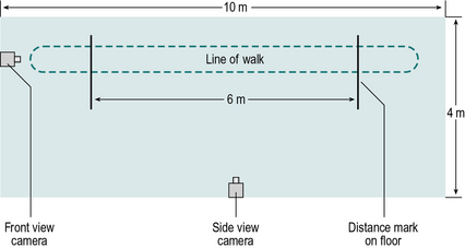
Fig. 4.1 • Layout of a small gait laboratory for visual gait analysis, video recording and measurement of the general gait parameters.
Some investigators permit subjects to choose their own walking speed, whereas others control the cycle time (number of steps in a set time) or the cadence (steps per minute), for example by asking them to walk in time with a metronome. The rationale for controlling the cadence is that many of the measurable parameters of gait vary with the walking speed and controlling this provides one means of reducing the variability. However, subjects are unlikely to walk naturally when trying to keep pace with a metronome, and patients with motor control problems may find it difficult or even impossible to walk at an imposed cadence. Zijlstra et al. (1995) found considerable differences in the gait of normal subjects between ‘natural’ walking and ‘constrained’ walking, in which the subject was required either to step in time with a metronome or to step on particular places on the ground. The answer to this dilemma is probably to accept the fact that subjects need to walk at different speeds and to interpret the data appropriately. This means that ‘normal’ values must be available for a range of walking speeds. An unresolved difficulty with this approach is that it may not be possible to get ‘normal’ values for very slow walking speeds, since normal individuals do not customarily walk very slowly and when asked to do so, some of the gait measurements become very variable (Brandstater et al., 1983).
Gait assessment
Simply observing the gait and noting abnormalities is of little value by itself. It needs to be followed by gait assessment, which is the synthesis of these observations with other information about the subject, obtained from the history and physical examination, combined with the intelligence and experience of the observer (Rose, 1983). Visual gait analysis is entirely subjective and the quality of the analysis depends on the skill of the person performing it. It can be an interesting exercise to perform visual gait analysis on people walking past in the street, but without knowing their clinical details it is easy to misinterpret what is wrong with them.
When performing any type of gait analysis, one thing that must be constantly borne in mind is that you are observing effects and not causes. Putting it another way, the observed gait pattern is not the direct result of a pathological process but the net result of a pathological process and the subject's attempts to compensate for it. The observed gait pattern is ‘what is left after the available mechanisms for compensation have been exhausted’ (Rose, 1983).
Examination by video recording
Historically the use of videotape was widespread in the 1990s, although now this is achieved by direct recording to a DVD, memory card or computer. This has provided one of the most useful enhancements to gait analysis in the clinical setting during recent years. This helps to overcome two of the limitations of visual gait analysis: the lack of a permanent record and the difficulty of observing high-speed events. In addition, it confers the following advantages:
1. It reduces the number of walks a subject needs to do
2. It makes it possible to show the subject exactly how they are walking
3. It makes it easier to teach visual gait analysis to someone else
4. It completes the picture in a gait report as seeing the patient is very meaningful while reading values of their analysis.
Gait examination by video recording is not an objective method, since it does not provide quantitative data in the form of numbers. However, it does provide a permanent record, which can be extremely valuable. The presence of an earlier recording of a subject's gait may be used to demonstrate to all concerned how much progress has been made, especially when this has occurred over a long period of time. In particular, it may convince a subject or family member that an improvement has occurred, when memory tells them that they are no better than they were several months ago!
When using video recording, the most practical system consists of camcorder(s). The majority of today's domestic camcorders are perfectly suitable for use in gait analysis, the requirements being a zoom lens, automatic focus, the ability to operate in normal room lighting and an electronically shuttered charge-coupled device (CCD) sensor, to eliminate blurring due to movement. These allow the user to freeze-frame the picture and to advance frame by frame through successive frames, or to play at a very slow speed to allow the user to observe movements which are too fast for the unaided eye. Many gait laboratories record video data directly into a computer, which may be synchronised with data collection from motion analysis systems (described later), or in some cases used to perform kinematic analysis depending on the number of cameras used. One limitation the majority of camcorders have is the frame rate at which they collect images, commonly 25–30 frames per second, which is not fast enough to pick up some subtleties of movement. However, with the correct software, it is possible to obtain a maximum sampling rate of 50 Hz for PAL (Phase Alternating Line) and 60 Hz for NTSC (National Television Standards Committee) based systems and new developments in video technology include lower cost, higher speed cameras.
In making a thorough visual gait analysis without the use of video recording, the subject needs to make repeated walks to confirm or refute the presence of each of the gait abnormalities listed in Table 4.1. If the subject is in pain or easily fatigued, this may be an unreasonable requirement and it may be difficult to achieve a satisfactory analysis. The use of video recording permits the subject to do a much smaller number of walks, as the person performing the analysis can watch the recording as many times as necessary.
Video recording facilitates the process of teaching visual gait analysis, in which the student often needs to see small abnormal movements which happen very quickly. It is much easier to see such movements if the gait can be examined in slow motion, with the instructor pointing out details on the television or computer monitor. The use of video recording also makes it possible to observe a variety of abnormal gaits which have been archived. A number of teaching animations are now available (Appendix 3).
Showing the subject a video recording of their own gait is not exactly ‘biofeedback’, since there is a time delay involved, but nonetheless it can be very helpful. When a therapist is working with a subject to correct a gait abnormality, the subject may gain a clearer idea of exactly what the therapist is concerned about if they can observe their own gait from the ‘outside’.
Although visual gait analysis using video recording is subjective, it is easy, at the same time, to derive some objective data. The general gait parameters (cycle time or cadence, stride length and speed) can be measured by a method which will be described in the next section. It is also possible to measure joint angles by using some form of on-screen digitiser such as Siliconcoach and Dartfish. Such measurements tend to be susceptible to some errors as the joints may not be viewed from precisely the correct angle, although reasonable joint movements of the lower limb in the sagittal plane and some joint movements in the coronal plane can be obtained.
Individual investigators will find their own ways of performing gait analysis using video recording. A common routine used involves the subject being asked to wear shorts or a swim suit, so that the majority of the leg is visible. It is important that the subject should walk as ‘normally’ as possible, so they are asked to wear their own indoor or outdoor shoes, with socks if preferred. Unless it would unduly tire the subject, it is a good idea to make one or two ‘practice’ walks, before starting video recording. Two camera positions are often used, one viewing from the side (sagittal plane) and the front (coronal plane) (Fig. 4.1). These are first adjusted to show the whole body from head to feet and the subject is recorded as they walk the length of the walkway in one direction. At the end of the walkway, the subject turns around, with a rest if necessary, and is recorded as they walk back again. The whole process may then be repeated with the cameras adjusted to show a close-up of the body from the waist down, or of the body segment of interest.
It is often helpful to mark the subject's skin, for example using an eyebrow pencil or whiteboard marker, to enhance the visibility of anatomical landmarks on the recording. Hillman et al. (1998) fitted subjects with surface-mounted ‘rotation indicators’, to improve the accuracy with which transverse plane rotations were estimated from video recording.
Subjects should not be able to see themselves on a monitor while they are walking, as this provides a distraction, particularly for children. The cameras should also be placed in a manner so that they are not a focus point. Whether they are shown the video recording afterwards is at the discretion of the investigator, although it is important to review the recording before the subject leaves, in case it needs to be repeated for some reason.
The analysis is performed by replaying the video recording, looking for specific gait abnormalities in the different views and interpreting what is seen in the light of the subject's history and physical examination. It is particularly helpful if two or more people work together to perform the analysis. Rose (1983) suggested that gait analysis should be based on the team approach, with discussion and hypothesis testing. As will be described in Chapter 5, hypothesis testing may involve an attempted modification of the gait, for instance by fitting an orthosis or by paralysing a muscle using local anaesthesia.
Temporal and spatial parameters during gait
Temporal and spatial parameters of gait, sometimes referred to as the general gait parameters, include cycle time (or stride time), stride length and speed. These provide the simplest form of objective gait evaluation (Robinson and Smidt, 1981) and may be made using only a stopwatch and a tape measure. Other temporal and spatial parameters of gait include, step time, double support time, single support time, step length, base width and foot angle. However these measurements require the use of specialist equipment which will be described in the next section.
Cycle time, stride length and speed tend to change together in most locomotor disabilities, so that a subject with a long cycle time will usually also have a short stride length and a low speed (speed being stride length divided by cycle time). The general gait parameters give a guide to the walking ability of a subject, but little specific information. They should always be interpreted in terms of the expected values for the subject's age and sex, such as those covered in Chapter 2. Figure 4.2 shows one way in which these data may be presented; the diamonds represent the 95% confidence limits for a normal subject of the same age and sex as the subject under investigation. Although cycle time is gradually replacing cadence in the gait analysis community, it is more convenient to use cadence on plots of this type, since abnormally slow gait will give values on the left-hand side of the graph for all three of the general gait parameters.
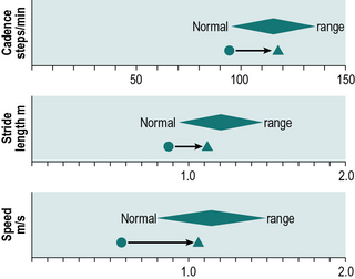
Fig. 4.2 • Display of the general gait parameters, with normal ranges appropriate for a patient's age and sex. Pre- and postoperative values for a 70-year-old female patient undergoing knee replacement surgery.
Cycle time or cadence
Cycle time or cadence may be measured with the aid of a stopwatch, by counting the number of individual steps taken during a known period of time. It is seldom practical to count for a full minute, so a period of 10 or 15 seconds is usually chosen. The loss of accuracy incurred by counting for such short periods of time is unlikely to be of any practical significance. The subject should be told to walk naturally and they should be allowed to get up to their full walking speed before the observer starts to count the steps. The cycle time is calculated using the formula:

The number ‘2’ allows for the fact that there are two steps per stride. The cadence is calculated using the formula:

The number ‘60’ allows for the fact that there are 60 seconds in a minute.
Stride length
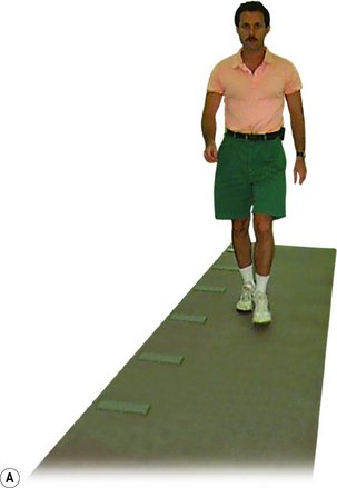
Stride length can be determined in two ways: by direct measurement or indirectly from the speed and cycle time. The simplest direct method of measurement is to count the strides taken while the subject covers a known distance. More useful methods include putting ink pads on the soles of the subject's shoes and walking on paper (Rafferty and Bell, 1995), using marker pens attached to shoes (Gerny, 1983) and a more messy option is to have the subject step with both feet in a shallow tray of talcum powder and then walk across a polished floor or along a strip of brown wrapping paper or coloured ‘construction paper’, leaving a trail of footprints. These may be measured, as shown in Figure 2.3, to derive left and right step lengths, stride length, walking base, toe out angle and some idea of the foot contact pattern. This investigation is able to provide a great deal of useful and surprisingly accurate information, for the sake of a few minutes of mopping up the floor afterwards! As an alternative to using talcum powder, felt adhesive pads, soaked in different coloured dyes, may be fixed to the feet (Rose, 1983). The subject walks along a strip of paper and leaves a pattern of dots, which give an accurate indication of the locations of both feet.
If both the cycle time and the speed have been measured, stride length may be calculated using the formula:

The equivalent calculation using cadence is:

The multiplication by ‘2’ converts steps to strides and by ‘60’ converts minutes to seconds. For accurate results, the cycle time and speed should be measured during the same walk. However, the simultaneous counting, measuring and timing may prove too difficult and the errors introduced by using data from different walks are not likely to be important, unless the subject's gait varies markedly from one walk to another.
Speed
The speed may be measured by timing the subject while he or she walks a known distance, for example between two marks on the floor or between two pillars in a corridor. The distance walked is a matter of convenience but somewhere in the region of 6–10 m (20–33 ft) is probably adequate. Again, the subject should be told to walk at their natural speed and they should be allowed to get into their stride before the measurement starts. The speed is calculated as follows:

General gait parameters from video recording
Determination of the general gait parameters from a video recording of the subject walking is easy, providing the recording shows the subject passing two landmarks whose positions are known. One simple method is to have the subject walk across two lines on the floor, a known distance apart, made with adhesive tape. Space should be allowed for acceleration before the first line and for slowing down after the second one. When the recording is replayed, the time taken to cover the distance is measured and the steps taken are counted. It is easiest to take the first initial contact beyond the start line as the point to begin both timing and counting and the first initial contact beyond the finish line as the point to end both timing and counting. The first step beyond the start line must be counted as ‘zero’, not ‘one’. This method of measurement is not strictly accurate, since the position of the foot at initial contact is an unknown distance beyond the start and finish line, but the errors introduced are unlikely to be significant. As mentioned above, this method can also be employed without the use of video recording.
Since the distance, the time and the number of steps are all known, the general gait parameters can be calculated using the formulae:


Measurement of temporal and spatial parameters during gait
A number of systems have been described which perform the automatic measurement of the timing of the gait cycle, sometimes called the temporal gait parameters. Such systems may be divided into two main classes: footswitches and instrumented walkways. Figure 4.3 shows typical data, which could be obtained from either type of system.
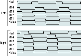
Fig. 4.3 • Output from footswitches under the heel, four metatarsals (MT1 to MT4) and hallux of both feet. The switch is ‘on’ (i.e. the area is in contact with the ground) when the line is high.
Footswitches
Footswitches are used to record the timing of gait. If one switch is fixed beneath the heel and one beneath the forefoot, it is possible to measure the timing of initial contact, foot flat, heel rise and toe off, and the duration of the stance phase (see Figs 2.2 and 4.3). Data from two or more strides make it possible to calculate cycle time and swing phase duration. If switches are mounted on both feet, the single and double support times can also be measured. The footswitches are usually connected through a trailing wire to a computer, although alternatively either a radio transmitter or a portable recording device may be used to collect the data and transfer them to the measuring equipment.
A footswitch is exposed to very high forces, which may cause problems with reliability. This has led to many different designs being tried over the years. A fairly reliable footswitch may be made from two layers of metal mesh, separated by a thin sheet of plastic foam with a hole in it. When pressure is applied, the sheets of mesh contact each other through the hole and complete an electrical circuit. Foot-switches are most conveniently used with shoes, although suitably designed ones may be taped directly beneath the foot. Small switches may also be mounted in an insole and worn inside the shoe. In addition to the basic heel and forefoot switches, further switches may be used in other areas of the foot, to give greater detail on the temporal patterns of loading and unloading. In addition to the home-made varieties, a number of companies also manufacture footswitches.
Instrumented walkways
An instrumented walkway is used to measure the timing of foot contact, the position of the foot on the ground, or both. Many different designs have been developed, usually individually built for a single laboratory. The descriptions which follow refer to typical designs, rather than to any particular system.
A conductive walkway is a gait analysis walkway which is covered with an electrically conductive substance, such as sheet metal, metal mesh or conductive rubber. Suitably positioned electrical contacts on the subject's shoes complete an electrical circuit. The conductive walkway is thus a slightly different method of implementing footswitches and provides essentially the same information. Again, the subject usually trails an electrical cable, which connects the foot contacts to a computer. The speed needs to be determined independently, typically by having the body of the subject interrupt the beams of two photoelectric cells, one at each end of the walkway, again connected to the computer. Timing information from the foot contacts is used to calculate the cycle time, and the combination of cycle time and speed may be used to calculate the stride length.
An alternative arrangement is to have the walkway itself contain a large number of switch contacts, which detect the position of the foot, as well as the timing of heel contact and toe off. This has the advantage that no trailing wires are required and the walkway can be used to measure both step lengths and the stride length. A number of commercial systems are available to make this type of measurement, often also providing some information on the magnitude of the forces between the foot and the ground. One such system, which is now in common use, is the ‘GAITRite’ (Bilney et al., 2003; Menz et al., 2004) (Fig. 4.4).
Camera-based motion analysis
Kinematics is the measurement of movement or, more specifically, the geometrical description of motion, in terms of displacements, velocities and accelerations. Kinematic systems are used in gait analysis to record the position and orientation of the body segments, the angles of the joints, and the corresponding linear and angular velocities and accelerations.
Following the pioneering work of Marey and Muybridge in the 1870s, photography remained the method of choice for the measurement of human movement for about 100 years, until it was replaced by electronic systems. Two basic photographic techniques were used: cine photography and multiple-exposure photography. Cine photography is achieved by the use of a series of separate photographs, taken in quick succession. Multiple exposure photography has existed in many different forms over the years. It is based on the use of a single photograph, or a strip of film on which a series of images are superimposed, sometimes with a horizontal displacement between each image and the next. The 1960s and 1970s saw the development of gait analysis systems based on optoelectronic techniques, including television, and these have now superseded photographic methods. The general principles of kinematic measurement are common to all systems and will be discussed before considering particular systems in detail.
General principles
Kinematic measurement may be made in either two dimensions or three. Three-dimensional measurements usually require the use of two or more cameras, although methods have been devised in which a single camera can be used to make limited three-dimensional measurements.
The simplest kinematic measurements are made using a single camera, in an uncalibrated system. Such measurements are fairly inaccurate but they may be useful for some purposes. Without calibration, it is impossible to measure distances accurately and such a system is usually used only to measure joint angles in the sagittal plane. The camera is positioned at right angles to the plane of motion and as far away as possible, to minimise the distortions introduced by perspective. To give a reasonable size image, with a long camera-to-subject distance, a ‘telephoto’ (long focal length) lens is used. The angles measured from the image are projections of three-dimensional angles onto a two-dimensional plane and any part of the angulation which occurs out of that plane is ignored. Commercial systems of this type are available for measuring joint angles from television images. Such measurements may be subject to yet another form of error, since the horizontal and vertical scales of a television image may be different.
A single-camera system can be used to make approximate measurements of distance, if some form of calibration object is used, such as a grid of known dimensions behind the subject. Measurement accuracy will be lost by any movement towards or away from the camera, but this effect can again be minimised if the camera is a long distance away from the subject, using a telephoto lens. Angulations of the limb segments, either towards or away from the camera, will also interfere with length measurements.
To achieve reasonable accuracy in kinematic measurement, it is necessary to use a calibrated three-dimensional system, which involves making measurements from more than one viewpoint. A detailed review of the technical aspects of the three-dimensional measurement of human movement was given in four companion papers by Cappozzo et al. (2005), Chiari et al. (2005), Leardini et al. (2005) and Della Croce et al. (2005). Although there are considerable differences in convenience and accuracy between cine film, video recording, television/computer and optoelectronic systems, the data processing for the different types of three-dimensional measurement systems is similar.
Most commercial kinematic systems use a three-dimensional calibration object, which is viewed by all the cameras, either simultaneously or in sequence. Computer software is used to calculate the relationship between the known three-dimensional positions of ‘markers’ on the calibration object and the two-dimensional positions of those markers in the fields of view of the different cameras. An alternative method of calibration is used by the Codamotion system, whose optoelectronic sensors are in fixed relation to each other, permitting the system to be calibrated in the factory.
When a subject walks in front of the cameras, the calibration process is reversed and three-dimensional positions are calculated for the markers fixed to the subject's limbs, so long as they are visible to at least two cameras. Data are collected at a series of time intervals known as ‘frames’. Most systems have an interval between frames of either 20 ms, 16.7 ms or 5 ms, corresponding to data collection frequencies of 50 Hz, 60 Hz or 200 Hz, with some systems now offering frame rates of up to 500 Hz and beyond. When a marker can be seen by only one camera, its three-dimensional position cannot be calculated, although it may be estimated by ‘interpolation’, using data from earlier and later frames.
All measurement systems, including the kinematic systems to be described, suffer from measurement errors. Measurement accuracy depends to a large extent on the field of view of the cameras, although it also differs somewhat between the different systems. The earlier systems had measurement errors of 2–3 mm in all three dimensions, throughout a volume large enough to cover a complete gait cycle (Whittle, 1982). Recently, design and (especially) calibration improvements have reduced typical errors to less than 1 mm. Some commercial systems claim to provide much higher accuracy than this, but the authors treat such claims with scepticism, particularly when applied to the measurement of moving markers under realistic gait laboratory conditions.
Technical descriptions of kinematic systems use, and sometimes misuse, the terms ‘resolution’, ‘precision’ and ‘accuracy’. In practical terms, resolution means the ability of the system to measure small changes in marker position. Precision is a measure of system ‘noise’, being based on the amount of variability there is between one frame of data and the next. For the majority of users, the most important parameter is accuracy, which describes the relationship between where the markers really are and where the system says they are!
Most commercial systems are sufficiently accurate to measure the positions of the limbs and the angles of the joints. However, the calculation of linear or angular velocity requires the mathematical differentiation of the position data, which magnifies any measurement errors. A second differentiation is required to determine acceleration, and a small amount of measurement ‘noise’ in the original data leads to wildly erratic and often unusable results for acceleration. The usual way of avoiding this problem is to smooth the position data, using a low-pass filter, before differentiation. This achieves the desired object but means that any genuinely high accelerations, such as that at the heelstrike transient, may be lost.
Thus, kinematic systems are good at measuring position but poorer at determining acceleration, because of the problems of differentiating even slightly noisy data. Conversely, accelerometers are good at measuring acceleration but poor at estimating position, because of the problems of integrating data with baseline drift. Really accurate data could be obtained by combining the two methods, using each to correct the other and calculating the velocity from both. Some research studies have been conducted using this combined approach.
As well as the errors inherent in measuring the positions of the markers, further errors are introduced because considerable movement may take place between a skin marker and the underlying bone. A few studies have been performed (e.g. Holden et al., 1997; Reinschmidt et al., 1997) in which steel pins were inserted into the bones of ‘volunteers’ (usually the investigators themselves) and the positions of skin markers compared with the positions of markers on the pins. The amount of skin movement revealed by such studies is generally somewhat worrying! The amount of error this causes in the final result depends on which parameter is being measured. For example, marker movement has little effect on the sagittal plane knee angle, because it causes only a small relative change in the length of fairly long segments, but it may cause considerable errors in transverse plane measurements or on measurements involving shorter segments, such as in the foot. In some cases, the magnitude of the error is greater than the measurement itself! Skin movement may also introduce errors in the calculation of joint moments and powers. A possibility for the future is to correct for marker movement, by estimating the movement relative to the underlying bone. A further error is introduced when the positions of the joints are estimated from anthropometric measures (e.g. leg length) and the positions of skin markers, particularly where it is possible to place the markers in the wrong position. Even for subjects with normal anatomy, these errors can be substantial; for patients with bony deformity, the errors may be even greater. For these reasons the development of marker sets and anatomical models has been at the forefront of the evolution of gait analysis alongside the ability of new motion analysis systems capable of coping with larger numbers of markers.
Camera-based systems
The use of video to augment visual gait analysis has already been described. Video recording may also be used as the basis for a kinematic system. This has considerable advantages in terms of cost, convenience and speed, although it is not as accurate, due to the poorer resolution of a video image and the sampling frequency compared with data collected from motion analysis cameras. Another considerable advantage, however, is that it is possible to automate the digitisation process using electronic processing of the image, especially if skin markers are used, which show up clearly against the background. A number of commercial systems are available, which can be used either as a two-dimensional system with a single camera, or as a three-dimensional system using two or more cameras. Most video recording systems use conventional television equipment, although high-speed systems are also available.
A number of different camera-based motion capture systems have been developed over the years. Although the systems differ in detail, the following description is typical. Reflective markers are fixed to the subject's limbs, either close to the joint centres or fixed to limb segments in such a way as to identify their positions and orientations. Close to the lens of each camera is an infrared or visible light source (Fig 4.5), which causes the markers to show up as very bright spots (Fig. 4.7).
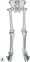
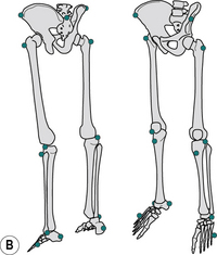
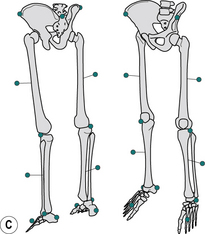
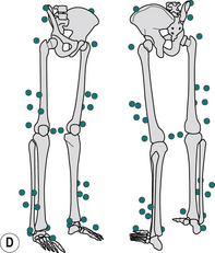
Fig. 4.5 • Common marker sets: (A) simple marker set; (B) Vaughan marker set; (C) Helen Hayes marker set; and (D) Calibrated Anatomical System Technique (CAST).
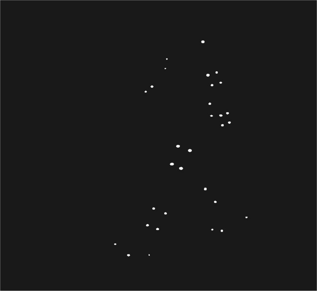
The markers are usually covered in ‘Scotchlite’, the material that makes road signs show up brightly when illuminated by car headlights. To avoid ‘smearing’, which occurs if the marker is moving, only a short exposure time is used. This may be achieved by one or more of the following:
1. Using stroboscopic illumination
2. Using a mechanical shutter on the camera
3. Using a charge-coupled device (CCD) camera, which is only enabled (i.e. activated) for a short interval during each frame.
If two or more cameras are used, much more accurate measurements can be made if they are synchronised. For normal purposes, frame rates of 50 Hz, 60 Hz or 200 Hz are used, although most systems are now able to collect at frame rates up to 500 Hz without loss of pixel resolution. Cameras are either connected via a special interface board, e.g. VICON or ‘daisy chained’, e.g. Qualisys (Fig. 4.6), both methods allow each frame to be synchronised. Most commercially available systems locate the ‘centroid’ or geometric centre of each marker within the camera image, but it is typically calculated using the edges of any bright spots in the field of view (Fig. 4.8). Because a large number of edges are used to calculate the position of the centroid, its position can be determined to a greater accuracy than the horizontal and vertical resolution of the image. This is known as making measurements with ‘subpixel accuracy’. Marker centroids may also be calculated using the optical density of all the pixels in the image, rather than just marker edges, again with an improvement in accuracy.
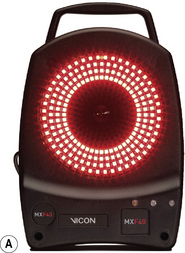
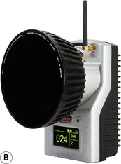
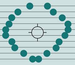
Fig. 4.8 • Location of marker centroid (open circle in centre) from the position on successive television lines of the leading and trailing edges of the marker image (solid circles).
The computer stores the marker centroids from each frame of data for each camera, but initially there is no way to associate a particular marker centroid with a particular physical marker. The process of identifying which marker image is which for each of the cameras, and of following the markers from one frame of data to the next, is known as ‘tracking’ (Fig. 4.9). The speed and convenience of this process differ considerably from one system to another. In the past this has been the least satisfactory aspect of motion capture systems, however many systems are now capable of real-time marker identification, allowing for much more straightforward and quicker analysis. Whichever method is used the end result of the tracking and three-dimensional reconstruction process is a computer file of three-dimensional marker positions.
Common marker sets
In order to calculate accurate joint kinetics it is essential to locate the centre of rotation of a joint in a repeatable manner through the definition of an anatomical frame. This issue was highlighted by Della Croce et al. (1999), who identified the errors associated with incorrect anatomical frame definition. Therefore the identification and modelling of joint centres has been key to the assessment of joint moments and powers. Joint centres are generally found by using palpable anatomical landmarks to define the medial-lateral axis of the joint. From these anatomical landmarks the centre of rotation is generally calculated in one of two ways: through the use of regression equations based on standard radiographic evidence or simply calculated as a percentage offset from the anatomical marker based on some kind of anatomical landmark (Bell et al., 1990; Cappozzo et al., 1995; Davis et al., 1991; Kadaba et al., 1989). We will now consider several commonly used marker sets which illustrate how improvements have continued to be made.
The simplest marker set involves directly fixing markers on the skin over a bony anatomical landmark close to the centre of rotation of a joint. The position and orientation of the limb segment is then defined by the straight line between the two markers (Fig. 4.5A). This method requires fewer markers and so theoretically has less interference with the movement pattern, but does not allow the calculation of axial rotation of the body segment. The anatomical landmarks generally used are: head of the fifth metatarsal, lateral malleolus, lateral epicondyle of the femur, greater trochanter and anterior superior iliac spine.
The Vaughan marker set consists of 15 markers on the lower limb and pelvis (Fig. 4.5B). This allows for more detail for the location of the knee joint centre by including a marker in the coronal plane on the tibial tuberosity. The inclusion of the heel marker allows a more appropriate functional reference for the long axis of the foot to be determined between this and the metatarsal heads with the pivot point of the foot determined by the malleoli markers. The inclusion of the sacral marker also allows for a more functional reference for pelvis inclination in the sagittal plane and a meaningful measurement of pelvic tilt. The anatomical landmarks used are: head of the fifth metatarsal, lateral malleolus, heel, tibial tuberosity, lateral femoral epicondyle, greater trochanter, anterior superior iliac spine and sacrum.
The conventional gait model, which is sometimes referred to as the Helen Hayes marker set (Fig. 4.5C), also includes a heel marker and the sacral marker for a more appropriate functional reference for the foot and pelvis. The conventional gait model marker set also includes tibial and femoral wands. Each of these comprises a single marker on a short stick, which is attached to a pad fixed to the segment using tape or bandage. These are not placed on any anatomical position as such and variations on the length of wand and positioning, anterior versus lateral, have been used. The inclusion of these wands allows femoral and tibial rotations to be quantified. The joint markers are placed on anatomical landmarks including: head of the second metatarsal, lateral malleolus, heel, lateral femoral epicondyle, anterior superior iliac spines and either the sacrum or on the posterior superior iliac spines.
The pelvis can be imagined as an equilateral triangle with its front edge formed by the line between the anterior superior iliac spine markers and mid-point of the posterior superior iliac spine markers. The hip joint centre is assumed to be fixed in relation to this triangle at a position estimated using regression equations. The thigh segment can be imagined as another equilateral triangle with its apex between the hip joint centre and the centre of the base at the knee joint axis. This is assumed to pass through the knee in the plane defined by a lateral knee marker, the thigh marker and the hip joint centre. The knee joint centre is defined as lying half the knee width along this axis from the knee marker. The tibia segment is modelled in a similar way to the femur. The foot is defined on the basis of the line between the ankle joint centre and the toe marker. This method does not require the inclusion of joint markers on the medial side and therefore can be potentially susceptible to errors in the estimation of the rotational axis as it uses a medial projection of both the knee and the ankle markers.
The Calibrated Anatomical System Technique (CAST, Fig. 4.5D), was first proposed by Cappozzo et al. (1995) to contribute towards standardising movement description in research labs and clinical centres for the pelvis and lower limb segments. This method involves identifying an anatomical frame for each segment through the identification of anatomical landmarks and segment tracking markers, or marker clusters. Anatomical markers are placed on both the lateral and medial aspects of joints to further improve the estimation of the joint centres. Marker clusters are placed on each body segment. The exact placement of the clusters does not matter, although positioning them on the distal third of the body segment is usual. At least three markers are required to track each segment position and orientation in six degrees of freedom (Cappozzo et al., 2005), however up to nine have been used. The usually accepted number is four or five markers per cluster, allowing for one or two markers to be lost. This is sometimes referred to as marker redundancy, i.e. if you lose a marker during tracking the model will still work. This method determines the position and orientation of each body segment separately, which then allows each joint to be assessed in what is referred to as six degrees of freedom. Six degrees of freedom is best thought of as: three orientations of rotation (i.e. flexion/extension, abduction/adduction, internal/external rotation), and three orientations of translation (i.e. anterior posterior and medial lateral translation, and compression and distraction), although the translational movements are more susceptible to soft tissue movement artefacts.
Active marker systems
Another type of kinematic system uses active markers, typically light-emitting diodes (LEDs), and an array of optoelectronic photo diodes. Among these systems the most common are Codamotion (Fig. 4.10) and Optotrack. Codamotion performs a correlation between the shadow cast on the array by a shadow mask of lines when the LED flashes and a software template of the shadow. This makes use of information from all photodiodes in the array to calculate the 3D marker positions. Optotrak forms a line image of the LED on a CCD Array using a toroidal lens to identify the position of the LED. Typically, these systems use invisible infra-red radiation, but for the sake of clarity, the word ‘light’ will be used in the following explanation.

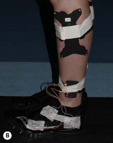
Fig. 4.10 • (A) Codamotion Opto-electronic movement analysis system (Charnwood Dynamics). (B) Codamotion Active LED marker clusters (Charnwood Dynamics).
In contrast, active markers produce light at a given frequency, so these systems do not require illumination and as such the markers are more easily identified and tracked (Chiari et al., 2005). The most frequently used active markers are those that emit an infra-red signal such as LEDs (Woltring, 1976). LEDs are attached to a body segment in the same way as passive markers, but with the addition of a power source and a control unit for each LED. Active markers can have their own specific frequency which allows them to be automatically detected. This leads to very stable real-time 3D motion tracking as no markers can be misidentified for adjacent markers. Active markers also have the advantage that they can be used outside, as passive marker systems are usually confined to indoors as they are sensitive to incandescent light and sunlight.
The LEDs are arranged to flash on and off in sequence, so that only one is illuminated at any instant of time. The photo diodes are thus able to locate each marker in turn, without the need for a ‘tracking’ procedure to determine which one is which. The penalty for this convenience is the need for the subject to carry a small power supply, with wires running to each of the markers. However Codamotion provide 4-marker clusters (Fig. 4.10) which are synchronized optically and require no wires. Problems may also occur because the photo diodes record not just the light from the LEDs, but any other light which falls on them. This may include stray ambient light, which is fairly easy to eliminate, and also reflections caused by the markers themselves, however in most systems these problems are largely eliminated.
Electrogoniometers and potentiometer devices
An electrogoniometer is a device for making continuous measurements of the angle of a joint. The output of an electrogoniometer is usually plotted as a chart of joint angle against time, as shown in Figure 2.5. However, if measurements have been made from two joints (typically the hip and the knee), the data may be plotted as an angle-angle diagram, also known as a ‘cyclogram’ (Fig. 4.11). This format allows the interaction between the two joints to be plotted on one graph and makes it possible to identify characteristic patterns, although these can sometimes be confusing to interpret.

Fig. 4.11 • Angle-angle diagram of the sagittal plane hip angle (horizontal axis) and knee angle (vertical axis). Initial contact is at the lower right. Normal subject; same data as Figure 2.5.
A rotary potentiometer is a variable resistor of the type used as a radio volume control, in which turning the central spindle produces a change in electrical resistance, which can be measured by an external circuit. It can be used to measure the angle of a joint if it is fixed in such a way that the body of the potentiometer is attached to one limb segment and the spindle to the other. The electrical output thus depends on the joint position and the device can be calibrated to measure the joint angle in degrees.
Although any joint motion could be measured by an electrogoniometer, they are most commonly used for the knee and less commonly for the ankle and hip. Fixation is usually achieved by cuffs, which wrap around the limb segment above and below the joint. The position of the potentiometer is adjusted to be as close to the joint axis as possible. A single potentiometer will only make measurements in one axis of the joint, but two or three may be mounted in different planes to make multiaxial measurements (Fig. 4.12). Trailing wires are usually used to connect the potentiometers to the measuring equipment, which is usually a computer. Concern has been expressed about the accuracy of measurement provided by these potentiometer devices, since they are subject to a number of possible types of error, described below.
1. The electrogoniometer is fixed by cuffs around the soft tissues, not to the bones, so that the output of the potentiometer does not exactly relate to the true bone-on-bone movement at the joint.
2. Some designs of electrogoniometer will only give a true measurement of joint motion if the potentiometer axis is aligned to the anatomical axis of the joint. This may not be achievable for three reasons:
3. A joint may, in theory, move with up to six degrees of freedom – that is, it may have angular motion about three mutually perpendicular axes and linear motion ‘translations’ in three directions. In practice, the linear motion is usually negligible, particularly at the hip and ankle, and most electrogoniometer systems simply ‘lose’ any motion which does occur, either through the elasticity of the mounting cuffs or through a sliding or ‘parallelogram’ mechanical linkage. However, where the electrogoniometer axis does not correspond exactly with the anatomical axis, larger linear motions will occur.
4. The output of the device gives a relative angle rather than an absolute one and it may be difficult to decide what limb angle should be taken as ‘zero’, particularly in the presence of a fixed deformity.
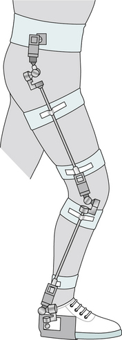
Fig. 4.12 • Subject wearing triaxial goniometers on hip, knee and ankle
(adapted from manufacturer's literature (Chattecx Corporation)).
Because of these problems, electrogoniometers are more popular in a clinical setting, in which great accuracy is not usually needed, than in the scientific laboratory. Chao (1980) addressed some of these problems in a defence of the use of potentiometer-based electrogoniometers in gait analysis.
Flexible strain gauge electrogoniometer
The flexible strain gauge electrogoniometer (Fig. 4.13), manufactured by Biometrics (Cwmfelinfach, Gwent, UK), consists of a flat, thin strip of metal, one end of which is fixed to the limb on each side of the joint being studied. The bending of the metal as the joint moves is measured by strain gauges and their associated electronics. Because of the way in which metal strips respond to bending, the output depends simply on the angle between the two ends, linear motion being ignored. To measure motion in more than one axis, a two-axis goniometer may be used, or two or three separate goniometers may be fixed around the joint, aligned to different planes.
Other electrogoniometers
With the increasing use of camera-based kinematic systems (see above), electrogoniometers are declining in popularity. Other designs which have been used in the past include mercury-in-rubber, in which the electrical resistance of a column of mercury in an elastic tube changes as the tube is stretched across a joint, and an optical system known as the polarised light goniometer.
Accelerometers
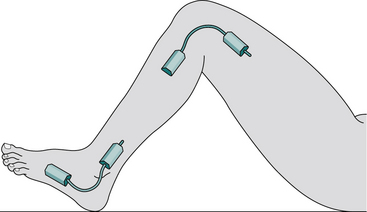
Accelerometers, as their name suggests, measure acceleration. Typically, they contain a small mass, connected to a stiff spring, with some electrical means of measuring the spring deflection when the mass is accelerated. The type of accelerometer used in gait analysis is usually very small, weighing only a few grams. It usually only measures acceleration in one direction, but more than one may be grouped together for two or three dimensional measurements. Solid-state accelerometers, built as integrated circuits, are also available. Because of their small size, they may be of value in gait analysis and also in providing feedback for future systems involving powered artificial limbs and orthoses. Typically, accelerometers have been used for gait analysis in one of two ways: either to measure transient events or to measure the motion of the limbs.
Measurement of transients with accelerometers
Accelerometers are suitable for measuring brief, high-acceleration events, such as the heelstrike transient. Johnson (1990) described the development of an accelerometer system to assess the performance of shock-attenuating footwear, which was made available commercially. The main difficulty with this type of measurement is in obtaining an adequate mechanical linkage between the accelerometer and the skeleton, since slippage occurs in both the skin and the subcutaneous tissues. On a few occasions, experiments have been performed with accelerometers mounted on pins, screwed directly into the bones of volunteers. Reviews of this subject were published by Collins and Whittle (1989) and Whittle (1999).
Measurement of motion with accelerometers
The use of accelerometers for the kinematic analysis of limb motion has been explored by a number of authors, notably Morris (1973). If the acceleration of a limb segment is known, a single mathematical integration will give its velocity and a second integration its position, provided both position and velocity are known at some point during the measurement period. However, these requirements, combined with the ‘drift’ from which accelerometers often suffer, have prevented them from coming into widespread use for this purpose. If the limb rotates as well as changing its position, which is usually the case, further accelerometers are needed to measure the angular acceleration.
Trunk accelerations have been used to measure the general gait parameters (Zijlstra and Hof, 2003). This is an extension of the principle behind the ‘pedometer’, often carried by hikers, which counts steps by measuring the vertical accelerations of the trunk.
Gyroscopes, magnetic fields and motion capture suits
It was suggested in the late twentieth century that gyroscopes could be used to measure the orientation of the body segments in space and that ‘rate-gyros’ could be used to measure angular velocity and acceleration. Gyroscopes were used on an experimental basis in some gait laboratories and the development of very small solid-state devices may make this a useful method of measurement in the future. Nene et al. (1999) used a gyroscope, in combination with several accelerometers, in a study of thigh and shank motion during the swing phase of gait. Several systems were also developed which could detect the position and orientation of a magnetometer sensor, which measures movement relative to magnetic fields. One example was a method for measuring motion of the lumbar spine developed by Pearcy and Hindle (1989), which used a source (transmitter) mounted on the sacrum and a sensor (receiver) over the first lumbar vertebra. Systems are also available in which the location of ultrasound transmitters, placed on the subject, is detected by an array of microphones.
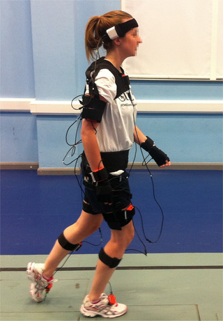
In the past 10 years considerable advances have been made in motion capture suits, at first in the gaming and animation industries, however these systems are now sensitive and reliable enough to be used in biomechanics and gait analysis. One such system is XSENS MVN motion capture suit (Fig. 4.14). This uses miniature three-dimensional (3D) gyroscopes, accelerometers and magnetometers. These systems require no cameras and do not require markers to be ‘seen’. Therefore they can be used indoors and outdoors regardless of lighting conditions. The combination of the three types of sensor allows the tracking of each segment in six degrees of freedom of up to 17 body segments. These systems do sometimes suffer from ‘drift’ and it is often difficult to obtain a global reference which prevents them being linked with force platforms, however, the relative movement of one body segment about another has been shown to be accurate.
Measuring force and pressure
Force platforms
The force platform, which is also known as a ‘forceplate’, is used to measure the ground reaction force as a subject walks across it (Fig. 4.15). Although many specialised types of force platform have been developed over the years, most clinical laboratories use a commercial platform, a ‘typical’ design being about 100 mm high, with a flat rectangular upper surface measuring 400 mm by 600 mm. To make the upper surface extremely rigid, it is either made of a large piece of metal or of a lightweight honeycomb structure. Within the platform, a number of transducers are used to measure tiny displacements of the upper surface, in all three axes, when force is applied to it. The electrical output of the platform may be provided as either eight channels or six. An eight-channel output consists of:
1. Four vertical signals, from transducers near the corners of the platform
2. Two fore–aft signals from the sides of the platform
3. Two side-to-side signals, from the front and back of the platform.
A six-channel output generally consists of:
1. Three force vector magnitudes
2. Three moments of force, in a coordinate system based on the centre of the platform.
Although it is possible to use the output signal from a force platform directly, for example by displaying it on an oscilloscope, it is much more usual to collect it into a computer, through an analogue-to-digital converter. Neither the eight-channel nor the six-channel force platform output is particularly convenient for biomechanical calculations and it is usual to convert the data to some other form. Regrettably, no standard has been established for the coordinate systems used for either kinetic or kinematic data.
Ideally, a force platform should be mounted below floor level, the upper surface being flush with the floor. If this is not possible, it is usual to build a slightly raised walkway, to accommodate the thickness of the platform. It is highly undesirable to have the subject step up onto the platform and then down off it again, since such a step could never be regarded as ‘normal’ walking. Force platforms are very sensitive to building vibrations and many early gait laboratories were built in basements, to reduce this form of interference. In the authors' opinion, this problem has been overemphasised, since although building vibrations can be seen in force platform data, they are negligible when compared with the magnitude of the signals recorded from subjects walking on the platform.
One problem which may be experienced when using force platforms is that of ‘aiming’. To obtain good data, the whole of the subject's foot must land on the platform. It is tempting to tell the subject where the platform is and to ask them to make sure that their footstep lands squarely on it. However, this is likely to lead to an artificial gait pattern, as the subject ‘aims’ for the platform. If at all possible, the platform should be disguised so that it is not noticeably different from the rest of the floor and the subject should not be informed of its presence. This may require a number of walks to be made, with slight adjustments in the starting position, before acceptable data can be obtained.
Where it is required to record from both feet, the relative positioning of two force platforms can be a considerable problem. There is no single arrangement which is satisfactory for all subjects, and some laboratories have designed systems in which one or both platforms can be moved, to suit the gait of individual subjects. Figure 4.16 shows the arrangement used in a number of laboratories, which is a reasonable compromise for studies on adults but is unsatisfactory when the stride length is either very short or very long. For subjects who have a very short stride length, such as children or patients with disorders such as multiple sclerosis, better results may be obtained if the platforms are mounted with their shorter dimensions in the direction of the walk. Alternatively, the direction of the walk may be altered, to cross the platforms diagonally. Despite these strategies, the problem may be insoluble. For example, Gage et al. (1984) observed that ‘force plate data were discounted because the smaller children frequently stepped on the same platform twice because of their short stride lengths’. Some laboratories improve their chances of obtaining good data by using three or four force platforms.

Fig. 4.16 • Typical arrangement of two force platforms for use in studies of adults (dimensions in mm).
It is often impossible to get the whole of one foot on one force platform and the whole of the other foot on the other one, without also having unwanted additional steps on one or other platform. To some extent, computer software can be used to ‘unscramble’ the data when both feet have stepped on one platform but, more commonly, it is necessary to use the data from only one foot at a time.
The usual methods of displaying force platform data are:
1. Individual components, plotted against time (see Fig. 2.20)
2. The ‘butterfly diagram’ (see Fig. 2.9)
3. The centre of pressure (see Figs 2.21).
In the latter case, if it is required to superimpose a foot outline in the correct position on the plot, it is necessary also to measure the position of the foot on the force platform, for example by using talcum powder.
A number of things have to be borne in mind when interpreting force platform data. Firstly, although the foot is the only part of the body in contact with the platform, the forces which are transmitted by the foot are derived from the mass and inertia of the whole body. The force platform has been described as a ‘whole-body accelerometer’; its output gives the acceleration in three-dimensional space of the centre of gravity of the body as a whole, including both the limb that is on the ground and the leg which is swinging through the air. This means that changes in total body inertia may swamp small changes in ground reaction force due to events occurring within the foot. For example, fairly high moments are recorded about the vertical axis during the stance phase of gait (Fig. 4.17). While these may be slightly modified by local events within the foot, they are mainly derived from the acceleration and retardation of the other leg, as it goes through the swing phase. The reaction to the forces responsible for this acceleration and retardation are transmitted to the floor through the stance phase leg and appear in the force platform output, principally as a torque about the vertical axis.

Fig. 4.17 • Moments about the vertical axis at the instantaneous centre of pressure, during the stance phase of gait. Normal subject, right leg. A positive moment occurs when the foot attempts to move clockwise relative to the floor.
When interpreting force platform data, it is also helpful to remember that force is equivalent to the rate of change of momentum. If two objects of identical mass are dropped onto a force platform from the same height, the one which bounces will produce a higher ground reaction force than one that does not. This may at first seem surprising, until it is realised that the change in momentum is twice as much for the object which bounces as it is for the one that does not. The onset and termination heelstrike transient, shown in Figure 2.23 (page 50), was recorded using a Bertec force platform which has a stiff but lightweight top plate, giving it a high frequency response. When measuring transients, it is important not to pass the data through a low pass filter. If the data are sampled using a computer analogue-to-digital converter, the sampling rate needs to be high enough to record the waveform accurately (the example in Fig. 2.23 used 1000 Hz).
Force platform data by themselves are of limited value in gait analysis. Nevertheless, some laboratories use them empirically, for example by looking for particular patterns in the ‘butterfly diagram’ (Rose, 1985) or comparing the heights of the different peaks and troughs. Forces, particularly peak vertical force may be looked at for changes over time with an intervention. An example is research on non-steroidal anti-inflammatory drugs used for osteoarthritis to determine if forces increase over time as pain decreases. Some inferences can also be made from the shapes of the curves of the individual force components. For example, there is an association between stance phase flexion of the knee and a dip at mid-stance in the vertical component of force. However, the true value of the force platform is only appreciated when the ground reaction force data are combined with kinematic data. The combination provides a much more complete mechanical description of gait than either by itself and permits the calculation of joint moments and powers.
A number of workers have developed devices which are not force platforms but have the same function. Typically, they consist of a small number of force sensors, which are fixed to the sole of a shoe. As the subject walks, the electrical output gives the ground reaction force and the centre of pressure. Typically only the vertical component of the ground reaction force is measured, although at least one three-axis system has been described. The advantages claimed are:
1. The ability to measure multiple steps
3. No risk of stepping on the platform with both feet
4. No risk of or missing the platform, either partly or completely.
The disadvantages are the presence of the force sensors beneath the feet, and the associated wiring. Also, the coordinate system for the force measurements moves with the foot, in contrast to the room-based coordinate system used for kinematic data. This makes it very difficult to combine the two types of data, to perform a full biomechanical analysis.
Force platforms may also be used for balance testing and the measurement of postural sway, which are important in some forms of neurological diagnosis. For a complete analysis of the balance mechanism, however, it is necessary to provide some means whereby both the supporting surface and the visual environment may be moved relative to the subject.
Pressure beneath the foot
The measurement of the pressure beneath the foot is a specialised form of gait analysis, which may be of particular value in conditions in which the pressure may be excessive, such as diabetic neuropathy and rheumatoid arthritis. Lord et al. (1986) reviewed a number of such systems. Foot pressure measurement systems may be either floor mounted or in the form of an insole within the shoe. The SI unit for pressure is the pascal (Pa), which is a pressure of one newton per square metre. The pascal is inconveniently small, and practical measurements are made in kilopascals (kPa) or megapascals (MPa). For conversions between different units of measurement, see Appendix 2.
Lord et al. (1986) pointed out that when making measurements beneath the feet, it is important to distinguish between force and pressure (force per unit area). Some of the measurement systems measure the force (or ‘load’) over a known area, from which the mean pressure over that area can be calculated. However, the mean pressure may be much lower than the peak pressure within the area if high pressure gradients are present, which are often caused by subcutaneous bony prominences, such as the metatarsal heads.
A pitfall which must be borne in mind when making pressure measurements beneath the feet is that a subject will usually avoid walking on a painful area. Thus, an area of the foot which had previously experienced a high pressure and has become painful may show a low pressure when it is tested. However, this will not happen if the sole of the foot is anaesthetic, as commonly occurs in diabetic neuropathy. In this condition, very high pressures, leading to ulceration, may be recorded.
Typical pressures beneath the foot are 80–100 kPa in standing, 200–500 kPa in walking and up to 1500 kPa in some sporting activities. In diabetic neuropathy, pressures as high as 1000–3000 kPa have been recorded. To put these figures into perspective, the normal systolic blood pressure, measured at the feet in the standing position, is below 33 kPa (250 mmHg); applied pressures which are higher than this will prevent blood from reaching the tissues.
Glass plate examination
Some useful semi-quantitative information on the pressure beneath the foot can be obtained by having the subject stand on, or walk across, a glass plate, which is viewed from below with the aid of a mirror or television camera. It is easy to see which areas of the sole of the foot come into contact with the walking surface and the blanching of the skin gives an idea of the applied pressure. Inspection of both the inside and the outside of a subject's shoe will also provide useful information about the way the foot is used in walking; it is a good idea to ask patients to wear their oldest shoes when they come for an examination, not their newest ones!
Direct pressure mapping systems
A number of low-technology methods of estimating pressure beneath the foot have been described over the years. The Harris or Harris–Beath mat is made of thin rubber, the upper surface of which consists of a pattern of ridges of different heights. Before use, it is coated with printing ink and covered by a sheet of paper, after which the subject is asked to walk across it. The highest ridges compress under relatively light pressures, the lower ones requiring progressively greater pressures, making the transfer of ink to the paper greater in the areas of the highest pressure. This gives a semi-quantitative map of the pressure distribution beneath the foot. Other systems have also been described, in which the subject walks on a pressure-sensitive film, a sheet of aluminium foil or on something like a typist's carbon paper.
Pedobarograph
The pedobarograph uses an elastic mat, laid on top of an edge-lit glass plate. When the subject walks on the mat it is compressed onto the glass, which loses its reflectivity, becoming progressively darker with increasing pressure. This darkening provides the means for quantitative measurement. The underside of the glass plate is usually viewed by a television camera, the monochrome image being processed to give a ‘false-colour’ display, in which different colours correspond to different levels of pressure.
Force sensor systems
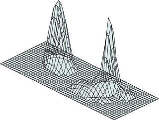
A number of systems have been described in which the subject walks across an array of force sensors, each of which measures the vertical force beneath a particular area of the foot. Dividing the force by the area of the cell gives the mean pressure beneath the foot in that area. Many different types of force sensor have been used, including resistive and capacitative strain gauges, conductive rubber, piezoelectric materials and a photoelastic optical system. A number of different methods have been used to display the output of such systems, including the attractive presentation shown in Figure 4.18.
In-shoe devices
The problem of measuring the pressure inside the shoe has been tackled in a number of centres. The main difficulties with this type of measurement are the curvature of the surface, a lack of space for the transducers and the need to run large numbers of wires from inside the shoe to the measuring equipment. Nonetheless, a number of commercial systems are now available, which may give clinically useful results. Details of such systems may be found on the internet (see Appendix 3).
Measuring muscle activity
Electromyography
Electromyography (EMG) is the measurement of the electrical activity of a contracting muscle, which is often referred to as the motor unit action potential (MUAP). Since it is a measure of electrical and not mechanical activity, the EMG cannot be used to distinguish between concentric, isometric and eccentric contractions, and the relationship between EMG activity and the force of contraction is far from straightforward. It is particularly good at determining the onset and termination of various muscles contraction during gait (Fig. 4.19). EMG signals have both magnitude and a frequency. The frequency range of the usable EMG signal is between 1 Hz and 500 Hz and the amplitude of the EMG signal varies between 1 μV and 1 mV. The concept of magnitude and frequency can be applied to any signal, but the best way to think about this is the parallel with sound waves. The magnitude of a sound wave is how loud the signal is, and the frequency is the pitch. So with EMG the magnitude of the signal relates to the amount of electric activity during a contraction and the frequency relates to the range of firing rates of all the motor units recorded. One of the most useful textbooks on the EMG is that by Basmajian (1974). The use of the EMG in the biomechanical analysis of movement was reviewed by Kleissen et al. (1998).
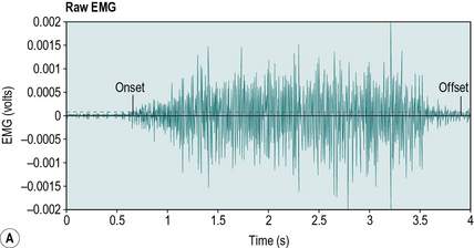
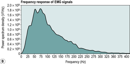
Fig. 4.19 • A) Timing of onset and termination of a muscle firing. (B) EMG signal power to frequency plot.
The EMG signal may be displayed in a number of ways. Clinical EMG biofeedback devices may display the magnitude of the signal by how many lights can be illuminated with a contraction. However for more scientific study the EMG signal is either displayed as a continuous line which oscillates up and down (Fig. 4.19A), or as a signal power to frequency plot (Fig. 4.19B). The three methods of recording the EMG are by means of surface, fine wire and needle electrodes. In gait analysis, EMG is usually measured with the subject walking, as opposed to the semi-static EMG measurements that are often made for neurological diagnosis.
Surface electrodes
Surface EMG is by far the most widely used method for gait analysis. Surface electrodes are fixed to the skin over the muscle, the EMG being recorded as the voltage difference between two electrodes. It is usually necessary also to have a grounding electrode, either nearby or elsewhere on the body. Since the muscle action potential reaches the electrodes through the intervening layers of fascia, fat and skin, the voltage of the signal is relatively small and it is usually amplified close to the electrodes, using a very small pre-amplifier. The EMG signal picked up by surface electrodes is the sum of the muscle action potentials from many motor units within the most superficial muscle or muscles. Most of the signal comes from within 25 mm of the skin surface, so this type of recording is not suitable for deep muscles such as the iliopsoas. When targeting the EMG of a particular muscle we sometimes pick up activity from adjacent muscles, this is referred to as ‘cross-talk’. Therefore it is sometimes safest to regard the signal from surface electrodes as being derived from muscle groups, rather than from individual muscles, although Õunpuu et al. (1997) showed that surface electrodes could satisfactorily distinguish between the three superficial muscle bellies of the quadriceps in children. There is often a change in the electrical baseline as the subject moves (‘movement artefact’) and there may also be electromagnetic interference, for example from nearby electrical equipment. The authors would recommend studying the wealth of information in the SENIAM guidelines (www.seniam.org) and also on the DelSys website (www.delsys.com).
Fine wire electrodes
Fine wire electrodes are introduced directly into a muscle, using a hypodermic needle which is then withdrawn, leaving the wires in place. They can be quite uncomfortable or even painful. The wire is insulated, except for a few millimetres at the tip. The EMG signal may be recorded in three different ways:
1. Between a pair of wires inserted using a single needle
The voltage recorded within the muscle is generally higher than that from surface electrodes, particularly if separate wires are used, and there is less interference from movement and from electromagnetic fields. The signal is derived from a fairly small region of a single muscle, generally from a few motor units only, a fact which must be taken into account when interpreting the data. Because it is an uncomfortable and invasive technique, fine-wire EMG is usually only performed on selected muscles, in patients in whom it is likely to be particularly useful.
Needle electrodes
Needle electrodes are generally more appropriate to physiological research than to gait analysis. A hypodermic needle is used, which contains an insulated central conductor. This records the EMG signal from a very local area within the muscle into which it is inserted, usually only a single motor unit.
Signal processing of EMG signals
Raw EMG
EMG signals are low voltage, and the signal can be hidden by other electrical noise. Therefore EMG signals have to be amplified to reduce the effect of this noise, typically between 1000 and 10 000 times to give a measurable signal. To decrease electrical interference the amplifiers can be positioned close to the electrodes, which reduces the length of wire that can pick up interference.
Often the EMG signal will oscillate on either side of a floating reference, this is referred to as low voltage offset, or bias. The way to remove bias is to find the mean value of the entire signal and then subtract this from the original signal, therefore pulling the data to a ‘zeroed’ position. The threshold of the signal can then be set to give information as to whether the muscle is firing or not. This gives an on/off measurement of whether the muscle is active or not, or muscle activity onset and termination.
Rectified, enveloped and integrated EMG
Rectification is required because the raw EMG signal (when the low voltage offset has been removed) oscillates positive and negative either side of the zero line, therefore if we were to try to find the mean value we would end up with zero. Rectification takes the entire signal and makes all the negative values in the signal positive. This can be achieved by first squaring the signal and then taking the square root. This is sometimes preferred when determining the threshold for the onset or termination of muscle contraction (Fig. 4.20A).
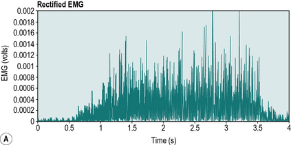
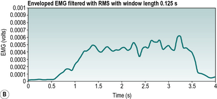
Enveloped EMG is a common method of showing the level of muscle activity which involves ‘filtering’ or ‘processing’ the EMG signal. A low pass filter is used which lets the lower frequencies through while stopping the higher frequencies. The practical upshot of this is a smoothing effect similar to that used in movement analysis. There is much debate as to how much this should be filtered; typical amounts of filtering used in the literature vary between 6 Hz and 25 Hz cut-off frequencies for a low pass filter. Another method of filtering is using the root mean square. The root mean square is calculated using a moving window and the calculation consists of three steps:
1. Squaring each data point in the signal
2. Determining an average value over a specified window length e.g. 0.125 seconds
3. Taking the square root (Fig. 4.20B).
Integrated EMG (iEMG) refers to the area under the full rectified EMG trace. This has been used as an indicator of work done by the muscle. From this the amount of ‘relative’ work done by a muscle group during push off during walking could be found if the events at the start and end of the push off were identified. Therefore iEMG would give us a single value for this period.
Limitations of EMG
The main problem with the use of any form of EMG is that it is at best only a semi-quantitative technique and gives little indication of the strength of contraction of individual muscles. Many attempts have been made over the years to make it more quantitative, with only limited success. The EMG signal is generally processed to provide a visible indication of muscle activity.
Despite its limitations, the information provided by EMG on the timing of muscle activation can be of considerable value in gait assessment. For example, one form of treatment in cerebral palsy is to transfer the tendon of a muscle to a different position, thereby altering the action of the muscle. When contemplating this type of surgery, it is essential to use EMG first, to make sure that the timing of muscular contraction is appropriate for its new role. It is also possible to determine any relative changes in activity due to immediate treatment, e.g. the use of orthoses, taping and bracing.
Measuring energy expenditure
The most accurate way of measuring the total amount of energy used in performing an activity such as walking is ‘whole-body calorimetry’, in which the subject is kept in an insulated chamber, from which the heat output of the body can be measured. This is, of course, quite impractical, except as a research technique. The most usual way of estimating energy expenditure is based on measuring the body's oxygen consumption. There are also less direct methods, using either mechanical calculations or the measurement of heart rate.
Oxygen consumption
The measurement of oxygen consumption requires an analysis of the subject's exhaled breath. If both the volume of exhaled air and its oxygen content are measured, the amount of oxygen consumed in a given time can be calculated. The amount of carbon dioxide produced can also be measured and the ratio of the carbon dioxide produced to the oxygen consumed (the ‘respiratory quotient’) provides information on the type of metabolism that is taking place (aerobic or anaerobic). Except under abnormal environmental conditions, it is not necessary to measure either the oxygen or the carbon dioxide in the inspired air, since these are almost constant.
The classic method of measuring oxygen consumption and carbon dioxide production is to fit the subject with a nose clip and mouthpiece and to collect the whole of the expired air in a large plastic or rubberised canvas ‘Douglas bag’ or a meteorological balloon. If the subject is walking, some means of following them around with the bag is needed. A small sample of the gas in the bag is then analysed, after which the volume of exhalate in the bag is measured. After correcting for temperature, air pressure and humidity, a very accurate estimate of oxygen consumption can be obtained. However, collecting the expirate in this way is uncomfortable for the subject and the technique is quite unsuitable for some patients.
A less cumbersome, though potentially slightly less accurate method again involves a nose clip and mouthpiece, but uses a portable system which performs continuous gas sampling and volume measurement, so that it is not necessary to collect the whole of the expirate. Either form of gas collection can be achieved using a facemask, rather than a mouthpiece and nose clip, although it may be very difficult either to prevent leakage or to detect leakage if it does occur. The use of a portable system with a facemask is routine in some gait analysis centres, who find that even children accept it well. Occasionally, studies of locomotion are made using a spirometer, in which the subject breathes in and out of an oxygen-filled closed system, which absorbs the exhaled carbon dioxide. Since spirometers are not usually portable, they are practical only when walking on a treadmill.
Whichever method is used this information can be presented in one of two ways, the energy expenditure per unit time and the energy expenditure per unit distance. Energy expenditure per unit time (Ew) shows an increase in the energy consumed by an individual with the square of the walking speed, which is usually reported as calorie/min or joules/sec (watt). This can be further developed by controlling for body mass, which allows comparison of the energy expenditure per kilogram between individuals of different mass (Fig. 4.21). The measurement of energy per unit distance walked (Em) provides a quantitative measure of energy economy. Figure 4.22 shows how the energy expenditure per metre walked varies with walking speed. When this value is at a minimum the individual is walking at their most efficient speed. Therefore we can determine that the most efficient walking speed is 1.33 m/s, 80 m/min, 4.7 km/h or 2.9 miles an hour, for normal able-bodied walking. Any increase or decrease in walking speed will cause an increase in the energy expenditure per metre walked and a reduction in efficiency (Corcoran and Brengelmann, 1970; Ralston, 1958). In this way the most efficient walking speed can be found for a particular individual and allows a useful comparison when studying pathological gait.

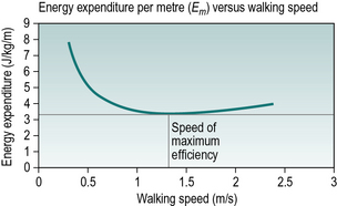
Heart rate monitoring
Rose (1983) stated that heart rate monitoring is a good substitute for the measurement of oxygen uptake, since a number of studies over the years have shown that there is a surprisingly close relationship between the two. Heart rate monitoring is certainly much easier to perform and there are a number of systems available, often based on detecting the pulsatile flow in the capillaries, for example in the finger. Another method of recording heart rate is to detect the electrocardiogram, using electrodes mounted on the chest. As a general rule, the energy consumption is related to the difference in heart rate between the resting condition and that measured during the exercise. Rather than attempting to relate the change in heart rate directly to energy consumption, some investigators use the ‘physiological cost index’ (PCI), which is said to be less sensitive to differences between individuals (Steven et al., 1983). It is calculated as follows:

The calculation must be made using consistent units, with the heart rate in beats per minute and the speed in metres per minute, or the heart rate in beats per second and the speed in metres per second. The measurement unit for the PCI is net beats per metre. Since the heart rate tends to be somewhat variable, small changes in PCI may not be significant; however, PCI gives a comparable pattern to the energy expenditure per metre (Em).
Mechanical calculations of energy expenditure
It was pointed out in Chapter 1 that the expenditure of metabolic energy does not result in the production of an equivalent amount of mechanical work. Indeed, in eccentric muscular activity, metabolic energy is used to absorb, rather than to generate, mechanical energy. Even when muscular contraction is used to do positive work, the efficiency of conversion is relatively low, as well as being variable and difficult to estimate. For these reasons, it is generally unsatisfactory to use mechanical calculations to estimate the total metabolic energy consumed in a complicated activity such as walking. Nonetheless, this method of estimating energy expenditure is used in some laboratories (Gage et al., 1984) and is known as the ‘estimated external work of walking’ (EEWW). Calculations of this type are more reliable for activities where the relationship between the muscular contraction and the mechanical output is extremely simple, such as in the concentric contraction of a single muscle.
Even though mechanical calculations are generally unsatisfactory for the estimation of the total energy consumption of the body, the measurement of the energy generation and transfer at individual joints may be of great value in gait analysis. Results of such measurements were given in Chapters 2 and 3. They may be made using combined kinetic/kinematic systems.
Combined kinetic/kinematic systems
When a kinematic system is combined with a force platform (which is a kinetic system), the capability of the combined system is greater than that of the sum of its component parts. The reason for this is that if the relationship is known between the limb segments and the ground reaction force vector, it is possible to perform ‘inverse dynamic’ calculations, in which the limb is treated as a mechanical system. While not all commercial systems provide the necessary software to make these calculations, there exists the potential to calculate the moments of force and the power generated or absorbed at all the major joints of the lower limb. Such calculations require knowledge of the masses and moments of inertia of the limb segments and the location of their centres of gravity. Direct measurements of these are clearly impossible, but published data, modified to suit the subject's anthropometry, give an acceptable approximation. It is common practice in such calculations to regard the foot as a single rigid object, although this simplification undoubtedly causes errors in calculating the ankle power.
A fully equipped clinical gait laboratory can be expected to possess, as a minimum, a combined kinetic/kinematic system, with ambulatory EMG (Fig. 4.23), as well as recording video. Equipment may also be available for measuring oxygen uptake or pressure beneath the feet. If the laboratory is also used for research, then further facilities and equipment may also be present.
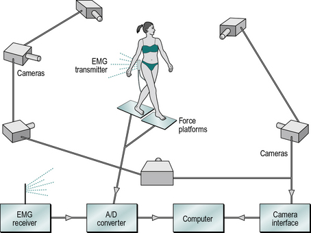
Fig. 4.23 • The gait analysis equipment used in the author's laboratory, with a six camera kinematic system, two force platforms and an EMG telemetry system.
One of the big problems with kinetic/kinematic systems is that they provide such a wealth of data that it may be very difficult to distinguish between those observations which are important and those which are not. Recent studies have used a number of mathematical, statistical and computational techniques in an attempt to address this problem (Chau, 2001a,b), some examples being multivariate analysis, principal component analysis, neural networks and the charmingly named ‘fuzzy systems’. It may be anticipated that in the future ‘expert systems’ will be available to draw the attention of clinicians to those aspects of a patient's gait most in need of attention. Another way of coping with this huge quantity of data is to reduce many different measurements to a single index. An example of this is the ‘normalcy index’ suggested by Schutte et al. (2000) as a method of quantifying a patient's disability and providing an outcome measure to gauge their response to treatment, which Romei et al. (2004) found to be ‘clinically applicable, reliable and easy to use’. This will be considered in more detail in Chapter 5.
Basmajian J.V. Muscles Alive: Their Functions Revealed by Electromyography. Baltimore, MD: Lippincott Williams & Wilkins; 1974.
Bell A., Pederson D., Brand R. A comparison of the accuracy of several hip centre location predication methods. J. Biomech.. 1990;23(6):617–621.
Bilney B., Morris M., Webster K. Concurrent related validity of the GAITRite walkway system for quantification of the spatial and temporal parameters of gait. Gait Posture. 2003;17:68–74.
Brandstater M.E., de Bruin H., Gowland C., et al. Hemiplegic gait: analysis of temporal variables. Arch. Phys. Med. Rehabil.. 1983;64:583–587.
Cappozzo A., Catani F., Croce U.D., Leardini A. Position and orientation in space of bones during movement: anatomical frame definition and determination. Clin. Biomech. (Bristol, Avon). 1995;10(4):171–178.
Cappozzo A., Della Croce U., Leardini A., et al. Human movement analysis using stereophotogrammetry. Part 1: Theoretical background. Gait Posture. 2005;21:186–196.
Chao E.Y.S. Justification of triaxial goniometer for the measurement of joint rotation. J. Biomech.. 1980;13:989–1006.
Chau T. A review of analytical techniques for gait data. Part 1: fuzzy, statistical and fractal methods. Gait Posture. 2001;13:49–66.
Chau T. A review of analytical techniques for gait data. Part 2: neural network and wavelet methods. Gait Posture. 2001;13:102–120.
Chiari L., Della Croce U., Leardini A., et al. Human movement analysis using stereophotogrammetry. Part 2: Instrumental errors. Gait Posture. 2005;21:197–211.
Collins J.J., Whittle M.W. Impulsive forces during walking and their clinical implications. Clin. Biomech. (Bristol, Avon). 1989;4:179–187.
Corcoran B. Oxygen uptake in normal and handicapped subjects, in relation to speed of walking beside velocity controlled cart. Arch. Phys. Med. Rehabil.. 1970;51:78–87.
Davis R., Ounpuu S., Tyburski D., Gage J. A gait data collection and reduction technique. Hum. Mov. Sci.. 1991;10:575–587.
Della Croce U., Cappozzo A., Kerrigan D.C. Pelvis and lower limb anatomical landmark calibration precision and its propagation to bone geometry and joint angles. Med. Biol. Eng. Comput.. 1999;37(2):155–161.
Della Croce U., Leardini A., Chiari L., et al. Human movement analysis using stereophotogrammetry. Part 4: Assessment of anatomical landmark misplacement and its effects on joint kinematics. Gait Posture. 2005;21:226–237.
Gage J.R., Fabian D., Hicks R., et al. Pre- and postoperative gait analysis in patients with spastic diplegia: a preliminary report. J. Pediatr. Orthop.. 1984;4:715–725.
Gerny K. A clinical method of quantitative gait analysis. Phys. Ther.. 1983;63:1125–1126.
Hillman S.J., Hazlewood M.E., Loudon I.R., et al. Can transverse plane rotations be estimated from video tape gait analysis? Gait Posture. 1998;8:87–90.
Holden J.P., Orsini J.A., Siegel K.L., et al. Surface movement errors in shank kinematics and knee kinetics during gait. Gait Posture. 1997;5:217–227.
Johnson G.R. Measurement of shock acceleration during walking and running using the shock meter. Clin. Biomech. (Bristol, Avon). 1990;5:47–50.
Kadaba M.P., Ramakrishnan H.K., Wootten M.E., Gainey J., Gorton G., Cochran G.V. Repeatability of kinematic, kinetic, and electromyographic data in normal adult gait. J. Orthop. Res.. 1989;7(6):849–860.
Kleissen R.F.M., Buurke J.H., Harlaar J., et al. Electromyography in the biomechanical analysis of human movement and its clinical application. Gait Posture. 1998;8:143–158.
Krebs D.E., Edelstein J.E., Fishman S. Reliability of observational kinematic gait analysis. Phys. Ther.. 1985;65:1027–1033.
Leardini A., Chiari L., Della Croce U., et al. Human movement analysis using stereophotogrammetry. Part 3: Soft tissue artifact assessment and compensation. Gait Posture. 2005;21:212–225.
Lord M., Reynolds D.P., Hughes J.R. Foot pressure measurement: a review of clinical findings. J. Biomed. Eng.. 1986;8:283–294.
Menz H.B., Latt M.D., Tiedemann A., et al. Reliability of the GAITRite walkway system for the quantification of temporo-spatial parameters of gait in young and older people. Gait Posture. 2004;20:20–25.
Morris J.R.W. Accelerometry – a technique for the measurement of human body movements. J. Biomech.. 1973;6:729–736.
Nene A., Mayagoitia R., Veltink P. Assessment of rectus femoris function during initial swing phase. Gait Posture. 1999;9:1–9.
Õunpuu S., DeLuca P.A., Bell K.J., et al. Using surface electrodes for the evaluation of the rectus femoris, vastus medialis and vastus lateralis in children with cerebral palsy. Gait Posture. 1997;5:211–216.
Pearcy M.J., Hindle R.J. New methods for the non-invasive three-dimensional measurement of human back movement. Clin. Biomech. (Bristol, Avon). 1989;4:73–79.
Ralston H.J. Energy speed relation and optimal speed during level walking. Int. Z. Angew. Physiol.. 1958;17:277.
Rafferty D., Bell F. Gait analysis – a semiautomated approach. Gait Posture. 1995;3(3):184.
Reinschmidt C., van den Bogert A.J., Lundberg A., et al. Tibiofemoral and tibiocalcaneal motion during walking: external vs. skeletal markers. Gait Posture. 1997;6:98–109.
Robinson J.L., Smidt G.L. Quantitative gait evaluation in the clinic. Phys. Ther.. 1981;61:351–353.
Romei M., Galli M., Motta F., et al. Use of the normalcy index for the evaluation of gait pathology. Gait Posture. 2004;19:85–90.
Rose G.K. Clinical gait assessment: a personal view. J. Med. Eng. Technol.. 1983;7:273–279.
Rose G.K. Use of ORLAU-Pedotti diagrams in clinical gait assessment. In: Whittle M., Harris D. Biomechanical Measurement in Orthopaedic Practice. Oxford: Clarendon Press; 1985:205–210.
Saleh M., Murdoch G. In defence of gait analysis. J. Bone Joint Surg. Br.. 1985;67:237–241.
Schutte L.M., Narayanan U., Stout J.L., et al. An index for quantifying deviations from normal gait. Gait Posture. 2000;11:25–31.
Steven M.M., Capell H.A., Sturrock R.D., et al. The physiological cost of gait (PCG): a new technique for evaluating nonsteroidal antiinflammatory drugs in rheumatoid arthritis. Br. J. Rheumatol.. 1983;22:141–145.
Whittle M.W. Calibration and performance of a three-dimensional television system for kinematic analysis. J. Biomech.. 1982;15:185–196.
Whittle M.W. Generation and attenuation of transient impulsive forces beneath the foot: a review. Gait Posture. 1999;10:264–275.
Whittle M.W., Levine D.F. Measurement of lumbar lordosis as a component of clinical gait analysis. Gait Posture. 1997;5:101–107.
Woltring H.J. Calibration and measurement in 3-dimensional monitoring of human motion by optoelectronic means. II. Experimental results and discussion. Biotelemetry. 1976;3(2):65–97.
Zijlstra W., Hof A.L. Assessment of spatio-temporal gait parameters from trunk accelerations during human walking. Gait Posture. 2003;18:1–10.
Zijlstra W., Rutgers A.W.F., Hof A.L., et al. Voluntary and involuntary adaptation of walking to temporal and spatial constraints. Gait Posture. 1995;3:13–18.
Bilney B., Morris M., Webster K. Concurrent related validity of the GAITRite walkway system for quantification of the spatial and temporal parameters of gait. Gait Posture. 2003;17:68–74.
Crosbie J., Vachalathiti R., Smith R. Patterns of spinal motion during walking. Gait Posture. 1997;5:6–12.
Klenerman L., Dobbs R.J., Weller C., et al. Bringing gait analysis out of the laboratory and into the clinic. Age Ageing. 1988;17:397–400.
Law H.T. Microcomputer-based, low cost method for measurement of spatial and temporal parameters of gait. J. Biomed. Eng.. 1987;9:115–120.
Law H.T., Minns R.A. Measurement of the spatial and temporal parameters of gait. Physiotherapy. 1989;75:81–84.
New York University. Lower Limb Orthotics. New York, NY: New York University Postgraduate Medical School; 1986.