
CHAPTER 16
Barry W. Connors
A neuron never works alone. Even in the most primitive nervous systems, all neurons participate in synaptically interconnected networks called circuits. In some hydrozoans (small jellyfish), the major neurons lack specialization and are multifunctional. They serve simultaneously as photodetectors, pattern generators for swimming rhythms, and motor neurons. Groups of these cells are monotonously interconnected by two-way electrical synapses into simple ring-like arrangements, and these networks coordinate the rhythmic contraction of the animal’s muscles during swimming. This simple neural network also has the flexibility to command defensive changes in swimming patterns when a shadow passes over the animal. Thus, neuronal circuits have profound advantages over unconnected neurons.
In more complex animals, each neuron within a circuit may have very specialized properties. By the interconnection of various specialized neurons, even a simple neuronal circuit may accomplish astonishingly intricate functions. Some neural circuits may be primarily sensory (e.g., the retina) or motor (e.g., the ventral horns of the spinal cord). Many circuits combine features of both, with some neurons dedicated to providing and processing sensory input, others to commanding motor output, and many neurons (perhaps most!) doing both. Neural circuits may also generate their own intrinsic signals, with no need for any sensory or central input to activate them. The brain does more than just respond reflexively to sensory input, as a moment’s introspection will amply demonstrate. Some neural functions—such as walking, running, breathing, chewing, talking, and piano playing—require precise timing, with coordination of rhythmic temporal patterns across hundreds of outputs. These basic rhythms may be generated by neurons and neural circuits called pacemakers because of their clock-like capabilities. The patterns and rhythms generated by a pacemaking circuit can almost always be modulated—stopped, started, or altered—by input from sensory or central pathways. Neuronal circuits that produce rhythmic motor output are sometimes called central pattern generators; we discuss these in a later section.
This chapter introduces the basic principles of neural circuits in the mammalian central nervous system (CNS). We describe a few examples of specific systems in detail to illuminate general principles as well as the diversity of neural solutions to life’s complex problems. However, this topic is enormous, and we have necessarily been selective and somewhat arbitrary in our presentation.
The function of a nervous system is to generate adaptive behaviors. Because different species face unique problems, we expect brains to differ in their organization and mechanisms. Nevertheless, certain principles apply to most nervous systems. It is useful to define various levels of organization. We can analyze a complex behavior—reading the words on this page—in a simple way, with progressively finer detail, down to the level of ion channels, receptors, messengers, and the genes that control them. At the highest level, we recognize neural subsystems and pathways (Chapter 10), which in this case include the sensory input from the retina (see Chapter 13) leading to the visual cortex, the central processing regions that make sense of the visual information, and the motor systems that coordinate movement of the eyes and head. Many of these systems can be recognized in the gross anatomy of the brain. Each specific brain region is extensively interconnected with other regions that serve different primary functions. These regions tend to have profuse connections that send information in both directions along most sensory/central motor pathways. The advantages of this complexity are obvious; while interpreting visual information, for example, it can be very useful to simultaneously analyze sound and to know where your eyes are pointing and how your body is oriented. (See Note: Levels of Organization of the Nervous System)
The systems of the brain can be more deeply understood by studying their organization at the cellular level. Within a local brain region, the arrangement of neurons and their synaptic connections is called a local circuit. A local circuit typically includes the set of inputs, outputs, and all the interconnected neurons that are essential to functions of the local brain region. Many regions of the brain are composed of a large number of stereotyped local circuits, almost modular in their interchangeability, that are themselves interconnected. Within the local circuits are finer arrangements of neurons and synapses sometimes called microcircuits. Microcircuits may be repeated numerous times within a local circuit, and they determine the transformations of information that occur within small areas of dendrites and the collection of synapses impinging on them. At even finer resolution, neural systems can be understood by the properties of their individual neurons (see Chapter 12), synapses, membranes, molecules (e.g., neurotransmitters and neuromodulators), and ions as well as the genes that encode and control the system’s molecular biology.
One of the most fascinating things about the nervous system is the wide array of different local circuits that have evolved for different behavioral functions. Despite this diversity, we can define a few general components of local circuits, which we illustrate with two examples from very different parts of the CNS: the ventral horn of the spinal cord and the cerebral neocortex. Some of the functions of these circuits are described in subsequent sections; here, we examine their cellular anatomy.
All local circuits have some form of input, which is usually a set of axons that originate elsewhere and terminate in synapses within the local circuit. A major input to the spinal cord (Fig. 16-1) is the afferent sensory axons in the dorsal roots. These axons carry information from somatic sensory receptors in the skin, connective tissue, and muscles (see Chapter 15). However, local circuits in the spinal cord also have many other sources of input, including descending input from the brain and input from the spinal cord itself, both from the contralateral side and from spinal segments above and below. Input to the local circuits of the neocortex (Fig. 16-2) is also easily identified; relay neurons of the thalamus send axons into particular layers of the cortex to bring a range of information about sensation, motor systems, and the body’s internal state. By far, the most numerous input to the local circuits of the neocortex comes from the neocortex itself—from adjacent local circuits, distant areas of cortex, and the contralateral hemisphere. These two systems illustrate a basic principle: local circuits receive multiple types of input.
Figure 16-1 Local circuits in the spinal cord. A basic local circuit in the spinal cord consists of inputs (e.g., sensory axons of the dorsal roots), interneurons (both excitatory and inhibitory), and output neurons (e.g., α motor neurons that send their axons through the ventral roots).
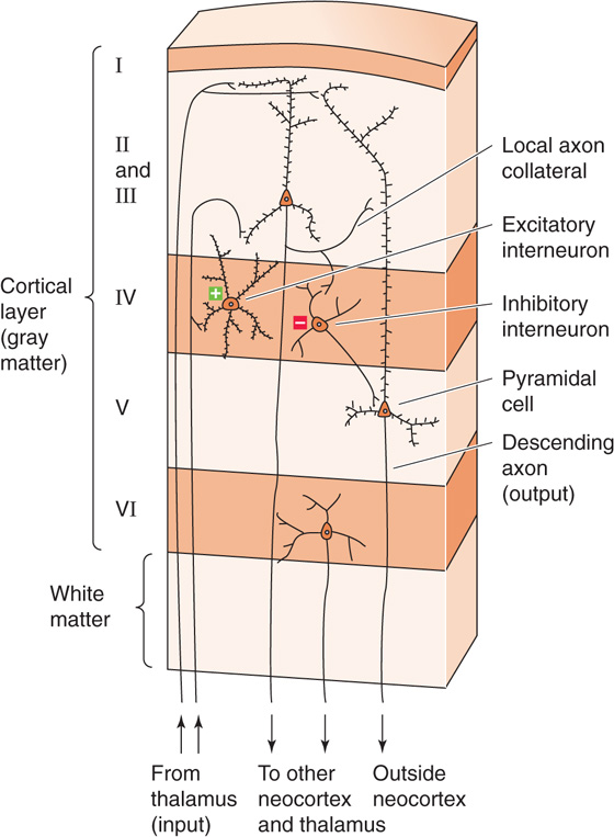
Figure 16-2 Local circuits in the neocortex. A basic local circuit in the neocortex consists of inputs (e.g., afferent axons from the thalamus), excitatory and inhibitory interneurons, and output neurons (e.g., pyramidal cells).
Output is usually achieved with a subset of cells known as projection neurons, or principal neurons, which send axons to one or more targets. The most obvious spinal output comes from the α motor neurons, which send their axons out through the ventral roots to innervate skeletal muscle fibers. Output axons from the neocortex come mainly from large pyramidal neurons in layer V, which innervate many targets in the brainstem, spinal cord, and other structures, as well as from neurons in layer VI, which make their synapses back onto the cells of the thalamus. However, as was true with input, most local circuits have multiple output. Thus, spinal neurons innervate other regions of the spinal cord and the brain, whereas neocortical circuits make most of their connections to other neocortical circuits.
Rare, indeed, is the neural circuit that has only input and output cells. Local processing is achieved by additional neurons whose axonal connections remain within the local circuit. These neurons are usually called interneurons, or intrinsic neurons. Interneurons vary widely in structure and function, and a single local circuit may have many different types. Both the spinal cord and neocortex have excitatory and inhibitory interneurons, interneurons that make very specific or widely divergent connections, and interneurons that either receive direct contact from input axons or process only information from other interneurons. In many parts of the brain, interneurons vastly outnumber output neurons. To take an extreme example, the cerebellum has ~1011 granule cells—a type of excitatory interneuron—which is more than the total number of all other types of neurons in the entire brain!
Numerous variations on the “principles” of local circuits outlined here may be mentioned. For example, a projection cell may have some of the characteristics of an interneuron, as when a branch of its output axon stays within the local circuit and makes synaptic connections. This branching is the case for the projection cells of both the neocortex (pyramidal cells) and the spinal cord (α motor neurons). On the other hand, some interneurons may entirely lack an axon and instead make their local synaptic connections through very short neurites or even dendrites. In some rare cases, the source of the input to a local circuit may not be purely synaptic but chemical (as with CO2-sensitive neurons in the medulla; see Chapter 32) or physical (as with temperature-sensitive neurons in the hypothalamus; see Chapter 59). Although the main neurons within a generic local circuit are wired in series (Figs. 16-1 and 16-2), local circuits, often in massive numbers, operate in parallel with one another. Furthermore, these circuits usually demonstrate a tremendous amount of crosstalk; information from each circuit is shared mutually, and each circuit continually influences its neighbors. Indeed, one of the things that makes analysis of local neural circuits so exceptionally difficult is that they operate in highly interactive, simultaneously interdependent, and expansive networks.
Reflexes are among the most basic of neural functions and involve some of the simplest neuronal circuits. A motor reflex is a rapid, stereotyped motor response to a particular sensory stimulus. Although the existence of reflexes was long appreciated, it was Sir Charles Sherrington who, beginning in the 1890s, first defined the anatomical and physiological bases for some simple spinal reflexes. So meticulous were Sherrington’s observations of reflexes and their timing that they offered him compelling evidence for the existence of synapses, a term he originated. (See Note: Sir Charles Scott Sherrington)
Reflexes are essential, if rudimentary, elements of behavior. Because of their relative simplicity, more than a century of research has taught us a lot about their biological basis. However, reflexes are also important for understanding of more complex behaviors. Intricate behaviors may sometimes be built up from sequences of simple reflexive responses. In addition, neural circuits that generate reflexes almost always mediate or participate in much more complex behaviors. Here we examine a relatively well understood example of reflex-mediating circuitry.
The CNS commands the body to move about by activating motor neurons, which excite skeletal muscles (Sherrington called motor neurons the final common path). Motor neurons receive synaptic input from many sources within the brain and spinal cord, and the output of large numbers of motor neurons must be closely coordinated to achieve even uncomplicated actions such as walking. However, in some circumstances, motor neurons can be commanded directly by a simple sensory stimulus—muscle stretch—with only the minimum of neural machinery intervening between the sensory cell and motor neuron: one synapse. Understanding of this simplest of reflexes, the stretch reflex or myotatic reflex, first requires knowledge of some anatomy.
Each motor neuron, with its soma in the spinal cord or brainstem, commands a group of skeletal muscle cells; a single motor neuron and the muscle cells that it synapses on are collectively called a motor unit (see Chapter 9). Each muscle cell belongs to only one motor unit. The size of motor units varies dramatically and depends on muscle function. In small muscles that generate finely controlled movements, such as the extraocular muscles of the eye, motor units tend to be small and may contain just a few muscle fibers. Large muscles that generate strong forces, such as the gastrocnemius muscle of the leg, tend to have large motor units with as many as several thousand muscle fibers. There are two types of motor neurons (see Table 12-1): α motor neurons innervate the main force-generating muscle fibers (the extrafusal fibers), whereas γ motor neurons innervate only the fibers of the muscle spindles. The group of all motor neurons innervating a single muscle is called a motor neuron pool (see Chapter 9).
When a skeletal muscle is abruptly stretched, a rapid, reflexive contraction of the same muscle often occurs. The contraction increases muscle tension and opposes the stretch. This stretch reflex is particularly strong in physiological extensor muscles—those that resist gravity—and it is sometimes called the myotatic reflex because it is specific for the same muscle that is stretched. The most familiar version is the knee jerk, which is elicited by a light tap on the patellar tendon. The tap deflects the tendon, which then pulls on and briefly stretches the quadriceps femoris muscle. A reflexive contraction of the quadriceps quickly follows (Fig. 16-3). Stretch reflexes are also easily demonstrated in the biceps of the arm and the muscles that close the jaw. Sherrington showed that the stretch reflex depends on the nervous system and requires sensory feedback from the muscle. For example, cutting of the dorsal (sensory) roots to the lumbar spinal cord abolishes the stretch reflex in the quadriceps muscle. The basic circuit for the stretch reflex begins with the primary sensory axons from the muscle spindles (see Chapter 15) in the muscle itself. Increasing the length of the muscle stimulates the spindle afferents, particularly the large group Ia axons from the primary sensory endings. In the spinal cord, these group Ia sensory axons terminate monosynaptically onto the α motor neurons that innervate the same (i.e., the homonymous) muscle from which the group Ia axons originated. Thus, stretching of a muscle causes rapid feedback excitation of the same muscle through the minimum possible circuit: one sensory neuron, one synapse, and one motor neuron.
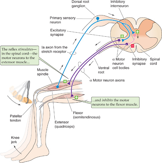
Figure 16-3 Knee jerk (myotatic) reflex. Tapping of the patellar tendon with a percussion hammer elicits a reflexive knee jerk caused by contraction of the quadriceps muscle: the stretch reflex. Stretching of the tendon pulls on the muscle spindle, exciting the primary sensory afferents, which convey their information through group Ia axons. These axons make monosynaptic connections to the α motor neurons that innervate the quadriceps, resulting in the contraction of this muscle. The Ia axons also excite inhibitory interneurons that reciprocally innervate the motor neurons of the antagonist muscle of the quadriceps (the flexor), resulting in relaxation of the semitendinosus muscle. Thus, the reflex relaxation of the antagonistic muscle is polysynaptic.
Monosynaptic connections account for much of the rapid component of the stretch reflex, but they are only the beginning of the story. At the same time the stretched muscle is being stimulated to contract, parallel circuits are inhibiting the α motor neurons of its antagonist muscles (i.e., those muscles that move a joint in the opposite direction). Thus, as the knee jerk reflex causes contraction of the quadriceps muscle, it simultaneously causes relaxation of its antagonists, including the semitendinosus muscle (Fig. 16-3). To achieve inhibition, branches of the group Ia sensory axons excite specific interneurons that inhibit the α motor neurons of the antagonists. This reciprocal innervation increases the effectiveness of the stretch reflex by minimizing the antagonistic forces of the antagonist muscles.
Skeletal muscle contains another sensory transducer in addition to the stretch receptor: the Golgi tendon organ (see Chapter 15). Tendon organs are aligned in series with the muscle; they are exquisitely sensitive to the tension within a tendon and thus respond to the force generated by the muscle rather than to muscle length. Tendon organs may respond during passive muscle stretch, but they are stimulated particularly well during active contractions of a muscle. The group Ib sensory axons of the tendon organs excite both excitatory and inhibitory interneurons within the spinal cord (Fig. 16-4). However, in most cases, this interneuron circuitry inhibits the muscle in which tension has increased and excites the antagonistic muscle; therefore, activity in the tendon organs usually yields effects that are almost the opposite of the stretch reflex. Under other circumstances, particularly in rapid movements, sensory input from Golgi tendon organs actually excites the motor neurons activating the same muscle. In general, reflexes mediated by the Golgi tendon organs serve to control the force within muscles and the stability of particular joints.
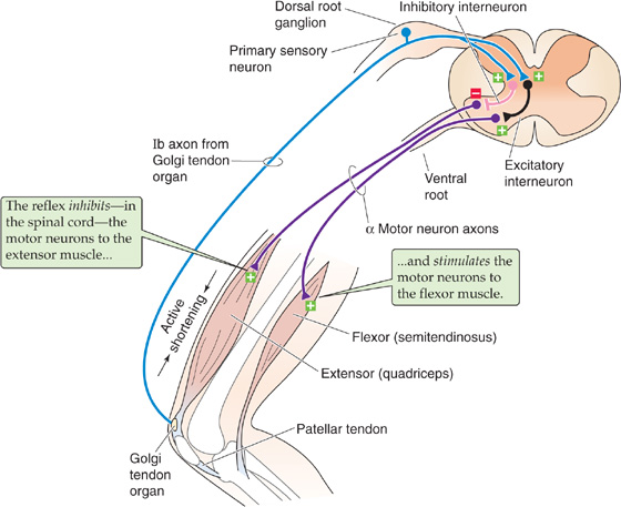
Figure 16-4 Golgi tendon organ reflex. Active contraction of the quadriceps muscle elicits a reflexive relaxation of this muscle and contraction of the antagonistic semitendinosus muscle: the inverse mytotatic reflex. Contraction of the muscle pulls on the tendon, which squeezes and excites the sensory endings of the Golgi tendon organ, which convey their information through group Ib axons. These axons synapse on both inhibitory and excitatory interneurons in the spinal cord. The inhibitory interneurons innervate α motor neurons to the quadriceps, relaxing this muscle. The excitatory interneurons innervate α motor neurons to the antagonistic semitendinosus muscle, contracting it. Thus, both limbs of the reflex are polysynaptic.
Sensations from the skin and connective tissue can also evoke strong spinal reflexes. Imagine walking on a beach and stepping on a sharp piece of shell (Fig. 16-5). Your response is swift and coordinated and does not require thoughtful reflection: you rapidly withdraw the wounded foot by activating the leg flexors and inhibiting the extensors. To keep from falling, you also extend your opposite leg by activating its extensors and inhibiting its flexors. This response is an example of a flexor reflex. The original stimulus for the reflex came from fast pain afferent neurons in the skin, primarily the group Aδ axons.

Figure 16-5 The flexor reflex. A painful stimulus to the right foot elicits a reflexive flexion of the right knee and an extension of the left knee: the flexor reflex. The noxious stimulus activates nociceptor afferents, which convey their information through group Aδ axons. These axons synapse on both inhibitory and excitatory interneurons. The inhibitory interneurons that project to the right side of the spinal cord innervate α motor neurons to the quadriceps and relax this muscle. The excitatory interneurons that project to the right side of the spinal cord innervate α motor neurons to the antagonistic semitendinosus muscle and contract it. The net effect is a coordinated flexion of the right knee. Similarly, the inhibitory interneurons that project to the left side of the spinal cord innervate α motor neurons to the left semitendinosus muscle and relax this muscle. The excitatory interneurons that project to the left side of the spinal cord innervate α motor neurons to the left quadriceps and contract it. The net effect is a coordinated extension of the left knee.
This bilateral flexor reflex response is coordinated by sets of inhibitory and excitatory interneurons within the spinal gray matter. Note that this coordination requires circuitry not only on the side of the cord ipsilateral to the wounded side but also on the contralateral side. That is, while you withdraw the foot that hurts, you must also extend the opposite leg to support your body weight. Flexor reflexes can be activated by most of the various sensory afferents that detect noxious stimuli. Motor output spreads widely up and down the spinal cord, as it must to orchestrate so much of the body’s musculature into an effective response. A remarkable feature of flexor reflexes is their specificity. Touching of a hot surface, for example, elicits reflexive withdrawal of the hand in the direction opposite the side of the stimulus, and the strength of the reflex is related to the intensity of the stimulus. Unlike simple stretch reflexes, flexor reflexes coordinate the movement of entire limbs and even pairs of limbs. Such coordination requires precise and widespread wiring of the spinal interneurons.
Axons descend from numerous centers within the brainstem and the cerebral cortex and terminate primarily onto the spinal interneurons, with some direct input to the motor neurons. This descending control is essential for all conscious (and much unconscious) command of movement, a topic beyond the scope of this chapter. Less obvious is that the descending pathways can alter the strength of reflexes. For example, to heighten an anxious patient’s stretch reflexes, a neurologist will sometimes ask the patient to perform the Jendrassik maneuver. The patient clasps his or her hands together and pulls; while the patient is distracted with that task, the examiner tests the stretch reflexes of the leg. Another example of the brain’s modulation of a stretch reflex occurs in catching a falling ball. If a ball were to fall unexpectedly from the sky and hit your outstretched hand, the force applied to your arm would cause a rapid stretch reflex—contraction in the stretched muscles and reciprocal inhibition in the antagonist muscles. The result would be that your hand slaps the ball back up into the air. However, if you anticipate catching the falling ball, for a short period around the time of impact (about ±60 ms), both your stretched muscles and the antagonist muscles contract! This maneuver stiffens your arm just when you need to squeeze that ball to not drop it. Stretch reflexes of the leg also vary dramatically during each step as we walk, thereby facilitating movement of the legs.
Like stretch reflexes, flexor reflexes can also be strongly affected by descending pathways. With mental effort, painful stimuli can be tolerated and withdrawal reflexes suppressed. On the other hand, anticipation of a painful stimulus may heighten the vigor of a withdrawal reflex when the stimulus actually arrives. Most of the brain’s influence on spinal circuitry is achieved by control of the many spinal interneurons.
Spinal reflexes are frequently studied in isolation from one another, and textbooks often describe them this way. However, under realistic conditions, many reflex systems operate simultaneously, and motor output from the spinal cord depends on interactions among them as well as on the state of controlling influences descending from the brain. It is now well accepted that reflexes do not simply correct for external perturbations of the body; in addition, they play a key role in the control of all movements.
The neurons involved in reflexes are the same neurons that generate other behaviors. Think again of the flexor response to the sharp shell—the pricked foot is withdrawn while the opposite leg extends. Now imagine that a crab pinches that opposite foot—you respond with the opposite pattern of withdrawal and extension. Repeat this a few times, crabs pinching you left and right, and you have achieved the basic pattern necessary for walking! Indeed, rhythmic locomotor patterns use components of these same spinal reflex circuits, as discussed next.
A common feature of motor control is the motor program, a set of structured muscle commands that are determined by the nervous system before a movement begins and that can be sent to the muscles with the appropriate timing so that a sequence of movements occurs without any need for sensory feedback. The best evidence for the existence of motor programs is that the brain or spinal cord can command a variety of voluntary and automatic movements, such as walking and breathing (see Chapter 32), even in the complete absence of sensory feedback from the periphery. The existence of motor programs certainly does not mean that sensory information is unimportant; on the contrary, motor behavior without sensory feedback is always different from that with normal feedback. The neural circuits responsible for various motor programs have been defined in a wide range of species. Although the details vary endlessly, certain broad principles emerge, even when vertebrates and invertebrates are compared. Here we focus on central pattern generators, well-studied circuits that underlie many of the rhythmic motor activities that are central to animal behavior.
Rhythmic behavior includes walking, running, swimming, breathing, chewing, certain eye movements, shivering, and even scratching. The central pattern generators driving each of these activities share certain basic properties. At their core is a set of cyclic, coordinated timing signals that are generated by a cluster of interconnected neurons. These basic signals are used to command as many as several hundred muscles, each precisely contracting or relaxing during a particular phase of the cycle; for example, with each walking step, the knee must first be flexed and then extended. Figure 16-6A shows how the extensor and flexor muscles of the left hind limb of a cat contract rhythmically—and out of phase with one another—while the animal walks. Rhythms must also be coordinated with other rhythms; for humans to walk, one leg must move forward while the other thrusts backward, then vice versa, and the arms must swing in time with the legs, but with the opposite phase. For four-footed animals, the rhythms are even more complicated and must be able to accommodate changes in gait (Fig. 16-6B). For coordination to be achieved among the various limbs, sets of central pattern generators must be interconnected. The motor patterns must also have great flexibility so that they can be altered on a moment’s notice—consider the adjustments necessary when one foot strikes an obstacle while walking or the changing motor patterns necessary to go from walking, to trotting, to running, to jumping. Finally, reliable methods must be available for turning the patterns on and off.
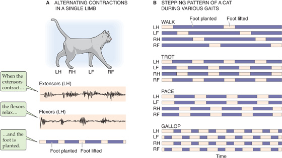
Figure 16-6 Rhythmic patterns during locomotion. A, The experimental tracings are electromyograms—extracellular recordings of the electrical activity of muscles—from the extensor and flexor muscles of the left hind limb of a walking cat. The pink bars indicate that the foot is lifted; purple bars indicate that the foot is planted. B, The walk, trot, pace, and gallop not only represent different patterns and frequencies of planting and lifting for a single leg but also different patterns of coordination among the legs. LF, left front; LH, left hind; RF, right front; RH, right hind. (Data from Pearson K: The control of walking. Sci Am 1976; 2:72-86.)
Motor System Injury
The motor control systems, because of their anatomy, are susceptible to damage from trauma or disease. The nature of a patient’s motor deficits often allows the neurologist to diagnose the site of neural damage with great accuracy. When injury occurs to lower parts of the motor system, such as motor neurons or their axons, deficits may be very localized. If the motor nerve to a muscle is damaged, that muscle may develop paresis (weakness) or complete paralysis (loss of motor function). When motor axons cannot trigger contractions, there can be no reflexes (areflexia). Normal muscles are slightly contracted even at rest—they have some tone. If their motor nerves are transected, muscles become flaccid (atonia) and eventually develop profound atrophy (loss of muscle mass) because of the absence of trophic influences from the nerves.
Motor neurons normally receive strong excitatory influences from the upper parts of the motor system, including regions of the spinal cord, the brainstem, and the cerebral cortex. When upper regions of the motor system are injured by stroke, trauma, or demyelinating disease, for example, the signs and symptoms are distinctly different from those caused by lower damage. Complete transection of the spinal cord leads to profound paralysis below the level of the lesion. This is called paraplegia when only both legs are selectively affected, hemiplegia when one side of the body is affected, and quadriplegia when the legs, trunk, and arms are involved. For a few days after an acute injury, there is also areflexia and reduced muscle tone (hypotonia), a condition called spinal shock. The muscles are limp and cannot be controlled by the brain or by the remaining circuits of the spinal cord. Spinal shock is temporary; after days to months, it is replaced by both an exaggerated muscle tone (hypertonia) and heightened stretch reflexes (hyperreflexia) with related signs—this combination is called spasticity. The mechanisms of spasticity are largely unknown, although the hypertonia is the consequence of tonically overactive stretch reflex circuitry, driven by spinal neurons that have become chronically hyperexcitable.
The central pattern generators for some rhythmic functions, such as breathing, are in the brainstem (see Chapter 32). Surprisingly, those responsible for locomotion reside in the spinal cord itself. Even with the spinal cord transected so that the lumbar segments are isolated from all higher centers, cats on a treadmill can generate well-coordinated stepping movements. Furthermore, stimulation of sensory afferents or descending tracts can induce the spinal pattern generators in four-footed animals to switch rapidly from walking, to trotting, to galloping patterns by altering not only the frequency of motor commands but also their pattern and coordination. During walking and trotting and pacing, the hind legs alternate their movements, but during galloping, they both flex and extend simultaneously (compare the leg patterns in Fig. 16-6B). Grillner and colleagues showed that each limb has at least one central pattern generator. If one leg is prevented from stepping, the other continues stepping normally. Under most circumstances, the various spinal pattern generators are coupled to one another, although the nature of the coupling must change to explain, for example, the switch from trotting to galloping patterns.
How do neural circuits generate rhythmic patterns of activity? There is no single answer, and different circuits use different mechanisms. The simplest pattern generators are single neurons whose membrane properties endow them with pacemaker properties that are analogous to those of cardiac muscle cells (see Chapter 21) and smooth muscle cells (see Chapter 9). Even when experimentally isolated from other neurons, pacemaker neurons may be able to generate rhythmic activity by relying only on their intrinsic membrane conductances. It is easy to imagine how intrinsic pacemaker neurons might act as the primary rhythmic driving force for sets of motor neurons that in turn command cyclic behavior. However, within vertebrates, although pacemaker neurons may contribute to some central pattern generators, they do not appear to be solely responsible for generating rhythms. Instead, they are embedded within interconnected circuits, and it is the combination of intrinsic pacemaker properties and synaptic interconnections that generates rhythms.
Neural circuits without pacemaker neurons can also generate rhythmic output. In 1911, Graham Brown proposed a pattern-generating circuit for locomotion. The essence of Brown’s half-center model is a set of excitatory and inhibitory interneurons arranged to inhibit one another reciprocally (Fig. 16-7). The half-centers are the two halves of the circuit, each commanding one of a pair of antagonist muscles. For the circuit to work, a tonic drive must be applied to the excitatory interneurons; this drive could come from axons originating outside the circuit or from the intrinsic excitability of the neurons themselves. Furthermore, some built-in mechanism must limit the duration of the inhibitory activity so that excitability can cyclically switch from one half-center to the other. Note that feedback from the muscles is not needed for the rhythms to proceed indefinitely. In fact, studies of more than 50 vertebrate and invertebrate motor circuits have confirmed that rhythm generation can continue in the absence of sensory information.
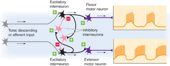
Figure 16-7 Half-center model for alternating rhythm generation in flexor and extensor motor neurons. Stimulation of the upper excitatory interneuron has two effects. First, the stimulated excitatory interneuron excites the motor neuron to the flexor muscle. Second, the stimulated excitatory interneuron excites an inhibitory interneuron, which inhibits the lower pathway. Stimulation of the lower excitatory interneuron has the opposite effects. Thus, when one motor neuron is active, the opposite one is inhibited.
The half-center model can produce rhythmic, alternating neural activity, but it is clearly too simplistic to account for most features of locomotor pattern generation. Analysis of vertebrate pattern generators is a daunting task, made difficult by the complexity of the circuits and the behaviors they control. In one of the most detailed investigations, Grillner and colleagues studied a simple model of vertebrate locomotion circuits: the spinal cord of the sea lamprey. Lampreys are among the simplest fish, and they swim with undulating motions of their body by using precisely coordinated waves of body muscle contractions. At each spinal segment, muscle activity alternates—one side contracts as the other relaxes. As in mammals, the rhythmic pattern is generated within the spinal cord, and neurons in the brainstem control the initiation and speed of the patterns. The basic pattern-generating circuit for the lamprey spinal cord is repeated in each of the animal’s 100 or so spinal segments.
The lamprey pattern-generating circuit improves on the half-center model in three ways. The first is sensory feedback. The lamprey has two kinds of stretch receptor neurons in the lateral margin of the spinal cord itself. These neurons sense stretching of the cord and body, which occurs as the animal bends during swimming. One type of stretch receptor excites the pattern generator interneurons on that same side and facilitates contraction, whereas the other type inhibits the pattern generator on the contralateral side and suppresses contraction. Because stretching occurs on the side of the cord that is currently relaxed, the effect of both stretch receptors is to terminate activity on the contracted side of the body and to initiate contraction on the relaxed side.
The second improvement of the lamprey circuit over the half-center model is the interconnection of spinal segments, which ensures the smooth progression of contractions down the length of the body, so that swimming can be efficient. Specifically, each segment must command its muscles to contract slightly later than the one anterior to it, with a lag of ~1% of a full activity cycle for normal forward swimming. Under some circumstances, the animal can also reverse the sequence of intersegment coordination to allow it to swim backward!
A third improvement over the half-center model is the reciprocal communication between the lamprey spinal pattern generators and control centers in the brainstem. Not only does the brainstem use numerous pathways and transmitters to modulate the generators, but the spinal generators also inform the brainstem of their activity.
The features outlined for swimming lampreys are relevant to walking cats and humans. All use spinal pattern generators to produce rhythms. All use sensory feedback to modulate locomotor rhythms (in mammals, feedback from muscle, joint, and cutaneous receptors is all-important). All coordinate the spinal pattern generators across segments, and all maintain reciprocal communication between spinal generators and brainstem control centers.
We have already seen that the spinal cord can receive sensory input, integrate it, and produce motor output that is totally independent of the brain. The brain also receives this sensory information and uses it to control the motor activity of the spinal reflexes and central pattern generators. How does the brain organize this sensory input and motor output? In many cases, it organizes these functions spatially by use of maps.
In everyday life, we use maps to represent spatial locations. You may use endless ways to construct a map, depending on which features of an area you want to highlight and what sort of transformation you make as you take measurements from the source (the thing being mapped) and place them on the target (the map). Maps of the earth may emphasize topography, the road system, political boundaries, the distributions of air temperature and wind direction, population density, or vegetation. A map is a model of a part of the world—and a very limited model at that. The brain also builds maps, most of which represent very selected aspects of our sensory information about the environment or the motor systems controlling our body. These maps can be spatial, or they can express nonspatial qualities of various sensory modalities (e.g., smell).
Almost all sensory receptors are laid out in planar sheets. In some cases, these receptor sheets are straightforward spatial maps of the sensory environment that they encode. For example, the somatic sensory receptors of the skin literally form a map of the body surface. Similarly, a tiny version of the visual scene is projected onto the mosaic of retinal photoreceptors. The topographies of other sensory receptor sheets represent qualities other than spatial features of the sensory stimuli. For example, the position of a hair cell along the basilar membrane in the cochlea determines the range of sound frequencies to which it will respond. Thus, the sheet of hair cells is a frequency map of sound rather than a map of the location of sounds in space. Olfactory and taste receptors also do not encode stimulus position; instead, because the receptor specificity varies topographically, the receptor sheets may be chemical maps of the types of stimuli. The most interesting thing about sensory receptor maps is that they often project onto many different regions of the CNS. In fact, each sensory surface may be mapped and remapped many times within the brain, the characteristics of each map being unique. In some cases, the brain constructs maps of stimulus features even when these features are not mapped at the level of the receptors themselves. Sound localization is a good example of this property (see the next section). Some neural maps may also combine the features of other neural maps, for example, overlaying visual information with auditory information.
Some of the best examples of brain maps are those of the visual fields. Figure 16-8A shows the basic anatomical pathway extending from the retina to the lateral geniculate nucleus of the thalamus and on to the primary visual cortex (area V1). Note that area V1 actually maps the visual thalamus, which in turn maps the retina, the first visuotopic map in the brain. Thus, the V1 map is sometimes referred to as a retinotopic map. Figure 16-8B shows how the visual fields are mapped onto cortical area V1. The first thing to notice is that the left half of the visual field is represented on the right cortex and the upper half of the visual field is represented on the lower portions of the cortex. This orientation is strictly determined by the system’s anatomy. For example, all the retinal axons from the left most halves of both eyes (which are stimulated by light from the right visual hemifield) project to the left half of the brain. Compare the red and blue pathways in Figure 16-8A. During development, each axon must therefore make an unerring decision about which side of the brain to innervate when it reaches the optic chiasm!
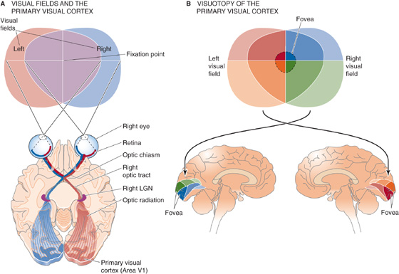
Figure 16-8 Visual maps. A, The right sides of both retinas (which sense the left visual hemifield) project to the left lateral geniculate, which in turn projects to the left primary visual cortex (area V1). B, The upper parts of the visual fields project to lower parts of the contralateral visual cortex, and vice versa. Although the fovea represents only a small part of the visual field, its representation is greatly magnified in the primary visual cortex, reflecting the large number of retinal ganglion cells that are devoted to the fovea. LGN, lateral geniculate nucleus.
The second thing to notice is that scaling of the visual fields onto the visual cortex—often called the magnification factor—is not constant. In particular, the central region of the visual fields—the fovea—is greatly magnified on the cortical surface. Behavioral importance ultimately determines mapping in the brain. Primates require vision of particularly high resolution in the center of their gaze; photoreceptors and ganglion cells are thus packed as densely as possible into the central retinal region (see Chapter 15). About half of the primary visual cortex is devoted to input from the relatively small fovea and the retinal area just surrounding it.
Understanding of a visual scene requires us to analyze many of its features simultaneously. An object may have shape, color, motion, location, and context, and the brain can usually organize these features to present a seamless interpretation, or image. The details of this process are only now being worked out, but it appears that the task is accomplished with the help of numerous visual areas within the cerebral cortex. Studies of monkey cortex by a variety of electrophysiological and anatomical methods have identified more than 25 areas, most of which are in the vicinity of area V1, that are mainly visual in function. According to recent estimates, humans devote almost half of their neocortex primarily to the processing of visual information. Several features of a visual scene, such as motion, form, and color, are processed in parallel and, to some extent, in separate stages of processing. The neural mechanisms by which these separate features are somehow melded into one image or concept of an object remain unknown, but they depend on strong and reciprocal interconnections between the visual maps in various areas of the brain.
The apparently simple topography of a sensory map looks much more complex and discontinuous when it is examined in detail. Many cortical areas can be described as maps on maps. Such an arrangement is especially striking in the visual system. For example, within area V1 of Old World monkeys and humans, the visuotopic maps of the two eyes remain segregated. In layer IV of the primary visual cortex, this segregation is accomplished by having visual input derived from the left eye alternate every 0.25 to 0.5 mm with visual input from the right. Thus, two sets of information, one from the left eye and one from the right eye, remain separated but adjacent. Viewed edge on, these left-right alternations look like columns (Fig. 16-9A), hence their name: ocular dominance columns. Viewed from the surface of the brain, this alternating left-right array of input looks like bands or zebra stripes (Fig. 16-9B). (See Note: David Hubel & Torsten Wiesel)
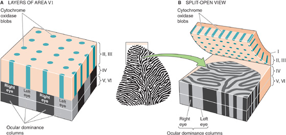
Figure 16-9 Ocular dominance columns and blobs in the primary visual cortex (area V1). A, Ocular dominance columns are shown as alternating black (right eye) and gray (left eye) structures in layer IV. The alternating light and dark bands are the result of an autoradiograph taken 2 weeks after injection of one eye with 3H-labeled proline and fucose. The 3H label moved from the optic nerve to neurons in the lateral geniculate and then to the axon terminals in the V1 cortex that are represented in this figure. The blobs are shown as teal-colored pegs in layers II and III. They represent the regular distribution of cytochrome oxidaserich neurons and are organized in pillar-shaped clusters. B, Cutting of the brain parallel to its surface, but between layers III and IV, reveals a polka-dot pattern of blobs in layer II/III and zebra-like stripes in layer IV. (Data from Hubel D: Eye, Brain and Vision. New York: WH Freeman, 1988.)
Superimposed on the zebra-stripe ocular dominance pattern in layer IV of the primary visual cortex, but quite distinct from these zebra stripes, layers II and III have structures called blobs. These blobs are visible when the cortex is stained for the mitochondrial enzyme cytochrome oxidase. Viewed edge on, these blobs look like round pegs (Fig. 16-9A). Viewed from the surface of the brain (Fig. 16-9A, B), the blobs appear as a polka-dot pattern of small dots that are ~0.2 mm in diameter.
Adjacent to the primary visual cortex (V1) is the secondary visual cortex (V2), which has, instead of blobs, a series of thick and thin stripes that are separated by pale interstripes. Some other higher order visual areas also have striped patterns. Whereas ocular dominance columns demarcate the left and right eyes, blobs and stripes seem to demarcate clusters of neurons that process and channel different types of visual information between areas V1 and V2 and pass them on to other visual regions of the cortex. For example, neurons within the blobs of area V1 seem to be especially attuned to information about color and project to neurons in the thin stripes of V2. Other neurons throughout area V1 are very sensitive to motion but are insensitive to color. They channel their information mainly to neurons of the thick stripes in V2.
One of the most famous depictions of a neural map came from studies of the human somatosensory cortex by Penfield and colleagues. Penfield stimulated small sites on the cortical surface of locally anesthetized but conscious patients during neurosurgical procedures; from their verbal descriptions of the position of their sensations, he drew a homunculus, a little person representing the somatotopy—mapping of the body surface—of the primary somatic sensory cortex (Fig. 16-10A). The basic features of Penfield’s map have been confirmed with other methods, including recording from neurons while the body surface is stimulated and modern brain imaging methods, such as positron emission tomography and functional magnetic resonance imaging. The human somatotopic map resembles a trapeze artist hanging upside down—the legs are hooked over the top of the postcentral gyrus and dangling into the medial cortex between the hemispheres, and the trunk, upper limbs, and head are draped over the lateral aspect of the postcentral gyrus.
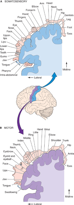
Figure 16-10 Somatosensory and motor maps. A, The plane of section runs through the postcentral gyrus of the cerebral cortex, shown as a blue band on the image of the brain. B, The plane of section runs through the precentral gyrus of the cerebral cortex, shown as a violet band on the image of the brain. (Data from Penfield W, Rasmussen T: The Cerebral Cortex of Man. New York: Macmillan, 1952.)
Two interesting features should be noticed about the somatotopic map in Figure 16-10A. First, mapping of the body surface is not always continuous. For example, the representation of the hand separates those of the head and face. Second, the map is not scaled like the human body. Instead, it looks like a cartoon character: the mouth, tongue, and fingers are very large, whereas the trunk, arms, and legs are tiny. As was the case for mapping of the visual fields onto the visual cortex, it is clear in Penfield’s map that the magnification factor for the body surface is not a constant but varies for different parts of the body. Fingertips are magnified on the cortex much more than the tips of the toes. The relative size of cortex that is devoted to each body part is correlated with the density of sensory input received from that part, and 1 mm2 of fingertip skin has many more sensory endings than a similar patch on the buttocks. Size on the map is also related to the importance of the sensory input from that part of the body; information from the tip of the tongue is more useful than that from the elbow. The mouth representation is probably large because tactile sensations are important in the production of speech, and the lips and tongue are one of the last lines of defense in deciding whether a morsel is a potential piece of food or poison.
The importance of each body part differs among species, and indeed, some species have body parts that others do not. For example, the sensory nerves from the facial whisker follicles of rodents have a huge representation on the cortex, whereas the digits of the paws receive relatively little. Rodent behavior explains this paradox. Most are nocturnal, and to navigate they actively sweep their whiskers about as they move. By touching their local environment, they can sense shapes, textures, and movement with remarkable acuity. For a rat or mouse, seeing things with its eyes is usually less important than “seeing” things with its whiskers.
As we have already seen for the visual system, other sensory systems usually map their information numerous times. Maps may be carried through many anatomical levels. The somatotopic maps in the cortex begin with the primary somatic sensory axons (see Table 12-1) that enter the spinal cord or the brainstem, each at the spinal segment appropriate to the site of the information that it carries. The sensory axons synapse on second-order neurons, and these cells project their axons into various nuclei of the thalamus and form synapses. Thalamic relay neurons in turn send their axons into the neocortex. The topographical order of the body surface (i.e., somatotopy) is maintained at each anatomical stage, and somatotopic maps are located within the spinal cord, the brainstem, and the thalamus as well as in the somatosensory cortex. Within the cortex, the somatic sensory system has several maps of the body, each unique and each concerned with different types of somatotopic information. Multiple maps are the rule in the brain.
Neural maps are not limited to sensory systems; they also appear regularly in brain structures that are considered to be primarily motor. Studies done in the 1860s by Fritsch and Hitzig showed that stimulation of particular parts of the cerebral cortex evokes specific muscle contractions in dogs. Penfield and colleagues generated maps of the primary motor cortex in humans (Fig. 16-10B) by microstimulating and observing the evoked movements. They noted an orderly relationship between the site of cortical stimulation and the body part that moved. Penfield’s motor maps look remarkably like his somatosensory maps, which lie in the adjacent cortical gyrus (Fig. 16-10A). Note that the sensory and motor maps are adjacent and similar in basic layout (legs represented medially and head laterally), and both have a striking magnification of the head and hand regions. Not surprisingly, there are myriad axonal interconnections between the primary motor and primary somatosensory areas. Functional magnetic resonance imaging of the human motor cortex shows that the motor map for hand movements is not nearly as simple and somatotopic as Penfield’s drawings might imply. Movements of individual fingers or the wrist, initiated by the individual, activate specific and widely distributed regions of motor cortex, but these regions also overlap one another. Rather than following an obvious somatotopic progression, it instead appears that neurons in the arm area of the motor cortex form distributed and co-operative networks that control collections of arm muscles. Other regions of the motor cortex also have a distributed organization when they are examined on a fine scale, although Penfield’s somatotopic maps still suffice to describe the gross organization of the motor cortex.
In other parts of the brain, motor and sensory functions may even occupy the same tissue, and precise alignment of the motor and sensory maps is usually the case. For example, a paired midbrain structure called the superior colliculus receives direct, retinotopic connections from the retina as well as input from the visual cortex. Accordingly, a spot of light in the visual field activates a particular patch of neurons in the colliculus. The same patch of collicular neurons can also command, through other brainstem connections, eye and head movements that bring the image of the light spot into the center of the visual field so that it is imaged onto the fovea. The motor map for orientation of the eyes is in precise register with the visual response map. In addition, the superior colliculus has maps of both auditory and somatosensory information superimposed on its visual and motor maps; the four aligned maps work in concert to represent points in polysensory space and help control an animal’s orienting responses to prominent stimuli (Fig. 16-11).
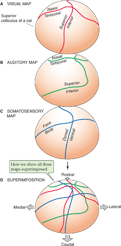
Figure 16-11 Polysensory space in the superior colliculus. In A, the illustration shows the representation of visual space that is projected onto the right superior colliculus of a cat. Note that visual space is divided into nasal versus temporal space and superior versus inferior space. In B and C, the illustrations show comparable auditory and somatosensory maps. In D, which shows the superimposition, note the approximate correspondence among the visual (red), auditory (green), and somatosensory (blue) maps, which are superimposed on one another. The motor map for orienting the eyes (not shown) is in almost perfect register with the visual map in A. (Data from Stein BE, Wallace MT, Meredith MA: Neural mechanisms mediating attention and orientation to multisensory cues. In Gazzaniga M [ed]: The Cognitive Neurosciences. Cambridge, MA: MIT Press, 1995.)
We have described a sample of the sensory and motor maps in the brain, but we are left to wonder just why neural maps are so ubiquitous, elaborate, and varied. What is the advantage of mapping neural functions in an orderly way? You could imagine other arrangements: spatial information might be widely scattered about on a neural structure, much as the bytes of one large digital file may be scattered across the surface of the hard disk of a computer. Various explanations may be proposed for the phenomenon of orderly mapping in the nervous system, although most remain speculations. Maps may be the most efficient way of generating nearest-neighbor relationships between neurons that must be interconnected for proper function. For example, the collicular neurons that participate in sensing stimuli 10 degrees up and 20 degrees to the left and other collicular neurons that command eye movements toward that point undoubtedly need to be strongly interconnected. Orderly collicular mapping enforces togetherness for those cells and minimizes the length of axons necessary to interconnect them. In addition, if brain structures are arranged topographically, neighboring neurons will be most likely to become activated synchronously. Neighboring neurons are very likely to be interconnected in structures such as the cortex, and their synchronous activity serves to reinforce the strength of their interconnections because of the inherent rules governing synaptic plasticity (see Chapter 13).
An additional advantage of mapping is that it may simplify establishment of the proper connections between neurons during development. For example, it is easier for an axon from neuron A to find neuron B if distances are short. Maps may thus make it easier to establish interconnections precisely among the neurons that represent the three sensory maps and one motor map in the superior colliculus. Another advantage of maps may be to facilitate the effectiveness of inhibitory connections. Perception of the edge of a stimulus (edge detection) is heightened by lateral connections that suppress the activity of neurons representing the space slightly away from the edge. If sensory areas are mapped, it is a simple matter to arrange the inhibitory connections onto nearby neurons and thereby construct an edge-detector circuit.
It is worth clarifying several general points about neural maps. “The map is not the territory, the word is not the thing it describes.”* In other words, all maps, including neural maps, are abstract representations of particular experimental measurements. A problem with neural maps is that different experimenters, using different methods, may sometimes generate quite different maps of the same part of the brain. As more and better refined methods become available, our understanding of these maps is evolving. Moreover, the brain itself muddies its maps. Maps of sensory space onto a brain area are not point-to-point representations. On the contrary, a point in sensory space (e.g., a spot of light) activates a relatively large group of neurons in a sensory region of the brain. However, such activation of many neurons is not due to errors of connectivity; the spatial dissemination of activity is part of the mechanism used to encode and to process information. The strength of activation is most intense within the center of the activated neuronal group, but the population of more weakly activated neurons may encompass a large portion of an entire brain. This diversity in strength of activation means that a point in sensory space is unlikely to be encoded by the activity of a single neuron, but instead it is represented by the distributed activity in a large population of neurons. Such a distributed code has computational advantages, and some redundancy also guards against errors, damage, and loss of information.
Finally, maps may change with time. All sensory and motor maps are clearly dynamic and can be reorganized rapidly and substantially as a function of development, behavioral state, training, or damage to the brain or periphery. Such changes are referred to as plasticity. Figure 16-12 illustrates two examples of dramatic changes in neocortical mapping, one sensory and one motor, after damage to peripheral nerves. In both cases, severing of a peripheral nerve causes the part of the map that normally relates to the body part served by this severed nerve to become remapped to another body part. Although the mechanisms of these reorganizations are not yet known, they probably reflect the same types of processes that underlie our ability to learn sensorimotor skills with practice and to adjust and improve after neural damage from trauma or stroke.
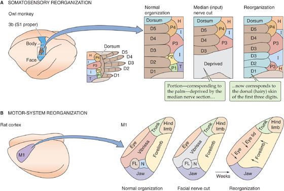
Figure 16-12 Plasticity of maps. A, The first panel, labeled “Normal organization,” shows the somatotopic organization of the right hand in the left somatosensory cortex of the monkey brain. The colors correspond to different regions of the hand (viewed from the palm side, except for portions labeled “dorsum”). The second panel shows (in gray) the territory that is deprived of input by sectioning of the median nerve. The third panel shows that the cortical map is greatly changed several months after nerve section. The nerve was not allowed to regrow, but the previously deprived cortical region now responds to the dorsal skin of D3, D2, and D1. Notice that responses to regions P1, P2, and T have disappeared; region I has encroached; and regions H and P3 have suddenly appeared at a second location. B, The first panel, labeled “Normal organization,” shows the somatotopic organization of the left motor cortex (M1) of the rat brain. The colors correspond to the muscles that control different regions of the body. The second panel shows (in gray) the territory that normally provides motor output to the facial nerve, which has been severed. The third panel shows that after several weeks, the deprived cortical territory is now remapped. Notice that the deprived territory that once evoked whisker movements now evokes eye, eyelid, and forelimb movements. (Data from Sanes J, Suner S, Donoghue JP: Dynamic organization of primary motor cortex output to target muscles in adult rats: Long-term patterns of reorganization following motor or mixed peripheral nerve lesions. Exp Brain Res 1990; 79:479-491.)
Neural circuits are very good at resolving time intervals, in some cases down to microseconds. One of the most demanding tasks of timing is performed by the auditory system as it localizes the source of certain sounds. Sound localization is an important skill, whether you are prey, predator, or pedestrian. Vertebrates use several different strategies for localization of sound, depending on the species, the frequency of the sound, and whether the task is to localize the source in the horizontal (left-right) or vertical (up-down) plane. In this subchapter, we briefly review general strategies of sound localization and then explain the mechanism by which a brainstem circuit measures the relative timing of low-frequency sounds so that the source of the sounds can be localized with precision.
Sound localization along the vertical plane (the degree of elevation) depends, in humans at least, on the distinctive shape of the external ear, the pinna. Much of the sound that we hear enters the auditory canal directly, and its energy is transferred to the cochlea. However, some sound reflects off the curves and folds of the pinna and tragus before it enters the canal and thus takes slightly longer to reach the cochlea. Notice what happens when the vertical direction of the sound changes. Because of the arcing shape of the pinna, the reflected path of sounds coming from above is shorter than that of sounds from below (Fig. 16-13). The two sets of sounds (the direct and, slightly delayed, the reflected) combine to create sounds that are slightly different on entering the auditory canal. Because of the interference patterns created by the direct and reflected sounds, the combined sound has spectral properties that are characteristic of the elevation of the sound source. This mechanism of vertical sound localization works well even with one ear at a time, although its precise neural mechanisms are not clear.
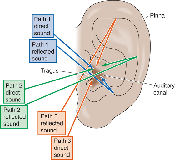
Figure 16-13 Detection of sound in the vertical plane. The detection of sound in the vertical plane requires only one ear. Regardless of the source of a sound, the sound reaches the auditory canal by both direct and reflected pathways. The brain localizes the source of the sound in the vertical plane by detecting differences in the combined sounds from the direct and reflected pathways.
Accurate determination of the direction of a sound along the horizontal plane (the azimuth) necessitates two working ears. Sounds must first be processed by the cochlea in each ear and then compared by neurons within the CNS to estimate horizontal direction. But what exactly is compared? For sounds that are relatively high in frequency (~2 to 20 xskHz), the important measure is the interaural (i.e., ear-to-ear) intensity difference. Stated simply, the ear facing the sound hears it louder than the ear facing away because the head casts a “sound shadow” (Fig. 16-14A). If the sound is directly to the right or left of the listener, this difference is maximal; if the sound is straight ahead, no difference is heard; and if the sound comes from an oblique direction, intensity differences are intermediate. Note that this system can be fooled. A sound straight ahead gives the same intensity difference (i.e., none) as a sound directly behind.

Figure 16-14 Sound detection in a horizontal plane. A, Two ears are necessary for the detection of sound in a horizontal plane. For frequencies between 2 kHz and 20 kHz, the CNS detects the ear-to-ear intensity difference. In this example, the sound comes from the right. The left ear hears a weaker sound because it is in the shadow of the head. B, For frequencies below 2 kHz, the CNS detects the ear-to-ear delay. In this example, the width of the head is 20 cm, and sound with a frequency of 200 Hz (wavelength of 172 cm) comes from the right. The peak of each sound wave reaches the left ear ~0.6 ms after it reaches the right.
The interaural intensity difference is not helpful at lower frequencies. Sounds below ~2 kHz have a wavelength that is longer than the width of the head itself. Longer sound waves are diffracted around the head, and differences in interaural intensity no longer occur. At low frequencies, the nervous system uses another strategy—it measures interaural delay (Fig. 16-14B). Consider a 200-Hz sound coming directly from the right. Its peak-to-peak distance (i.e., the wavelength) is ~172 cm, which is considerably more than the 20-cm width of the head. Each sound wave peak will reach the right ear ~0.6 ms before it reaches the left ear. If the sound comes from a 45-degree angle ahead, the interaural delay is ~0.3 ms; if it comes from straight ahead (or directly behind), the delay is 0 ms. Delays of small fractions of a millisecond are well within the capabilities of certain brainstem auditory neurons to detect. Sounds need not be continuous for the interaural delay to be detected. Sound onset or offset, clicks, or any abrupt changes in the sound give opportunities for interaural time comparisons. Obviously, measurement of interaural delay is subject to the same front-back ambiguity as interaural intensity, and indeed, it is sometimes difficult to distinguish whether a sound is in front of or behind your head.
How does the auditory system measure interaural timing? Surprisingly, to detect very small time differences, the nervous system uses a precise arrangement of neurons in space. Figure 16-15A summarizes the neuroanatomy of the first stages of central auditory processing within the brainstem. Notice that neurons in each of the cochlear nuclei receive information from only the ear on that one side, whereas neurons from the medial superior olivary (MSO) nucleus—and higher CNS centers—receive abundant input from both ears. Because horizontal sound localization requires input from both ears, we may guess that “direction-sensitive neurons” will probably be found somewhere central to the cochlear nuclei. When cochlear nucleus neurons are activated by auditory stimuli, their action potentials tend to fire with a particular phase relationship to the sound stimulus. For example, such a neuron might fire at the peak of every sound wave or at the peak of every fifth sound wave. That is, its firing is phase locked to the sound waves, at least for relatively low frequencies. Hence, cochlear neurons preserve the timing information of sound stimuli. Neurons in the MSO nucleus receive synaptic input from axons originating in both cochlear nuclei, so they are well placed to compare the timing (the phase) of sounds arriving at the two ears. Recordings from MSO neurons demonstrate that they are exquisitely sensitive to interaural time delay, and the optimal delay for superior olivary neurons varies systematically across the nucleus. In other words, the MSO nucleus has a spatial map of interaural delay. The olive also has a systematic map of sound frequency, so it simultaneously maps two qualities of sound stimuli.
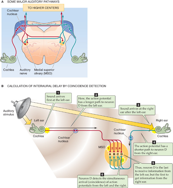
Figure 16-15 CNS processing of sounds. A, The figure shows a cross section of the medulla. After a sound stimulus to the cochlea, the cochlear nerve carries an action potential to the cochlear nucleus, which receives information only from the ear on the same side. However, higher auditory centers receive input from both ears. B, Neurons in the MSO nucleus are each tuned to a different interaural delay. Only when action potentials from the right and left sides arrive at the MSO neuron simultaneously does the neuron fire an action potential (coincidence detection). In this example, the two action potentials are coincident at MSO neuron D because the brief acoustic delay to the left ear is followed by a long neuronal conduction delay, whereas the long acoustic delay to the right ear is followed by a brief neuronal conduction delay.
In the brains of birds, and perhaps also in mammals, the tuning of MSO neurons to interaural delay seems to depend on neural circuitry that combines “delay lines” with “coincidence detection,” an idea first proposed by Jeffress in 1948. Delay lines are the axons from each cochlear nucleus; their length and conduction velocity determine how long it takes sound-activated action potentials to go from a cochlear nucleus to the axon’s presynaptic terminals onto MSO neurons (Fig. 16-15B). Axons from both the right and left cochlear nuclei converge and synapse onto a series of neurons in the MSO nucleus. However, each axon (each delay line) may take a different time to conduct its action potential to the same olivary neuron. The difference in conduction delay between the axon from the right side and that from the left side determines the optimal interaural delay for that particular olivary neuron. It is the olivary neuron that acts as the coincidence detector: only when action potentials from both the left and right ear axons reach the postsynaptic olivary neuron simultaneously (meaning that sound has reached the two ears at a particular interaural delay) is that neuron likely to receive enough excitatory synaptic transmitter to trigger an action potential. If input from the two ears arrives at the neuron out of phase, without coincidence in time, the neuron will not fire. All these postsynaptic superior olivary neurons are fundamentally the same: they fire when there is coincidence between input from the left and right. However, because neurons arrayed across the olive are mapped so that the axons connecting them have different delays, they display coincidence for different interaural delays. Thus, each is tuned to a different interaural delay and a different sound locale along the horizontal axis. The orderly arrangement of delay lines across the olive determines each of the neurons’ preferred delays (and thus sound location preferences) and leads to the orderly spatial mapping of sound direction.
The neural circuit we just described, which combines axonal delay lines and coincidence detection neurons, may not be the mechanism by which interaural timing is measured in mammalian brains. In the auditory system of gerbils, it appears that synaptic inhibition rather than delay lines generates the sensitivity of superior olivary neurons to interaural delay. It is possible that elements of both delay lines and inhibition are combined to optimize the measurement of timing in mammals.
Neural maps of sound localization are an interesting example of a sensory map that the brain must compute. This computed map contrasts with many other sensory maps that are derived more simply, such as by an orderly set of connections between the sensory receptor sheet (e.g., the retinal photoreceptors) and a central brain structure (e.g., the superior colliculus), as described in the preceding subchapter (Fig. 16-8). The cochlea does not have any map for sound location. Instead, the CNS localizes low-frequency sounds by calculating an interaural time-delay map, using information from both ears together. Other circuits can build a computed map of interaural intensity differences, which can be used for localization of high-frequency sounds (Fig. 16-14A). Once these two orderly sensory maps have been computed, they can be remapped onto another part of the brain by a simple system of orderly connections. For instance, the inferior colliculus receives parallel information on both timing delay and intensity difference; it transforms these two sets of information, combines them, and produces a complete map of sound direction. This combination of hierarchic (lower to high centers) and parallel information processing is probably ubiquitous in the CNS and is a general strategy for the analysis of much more complex sensory problems than those described here.
Books and Reviews
Bear MF, Connors BW, Paradiso MA: Neuroscience: Exploring the Brain, 2nd ed. Baltimore: Lippincott Williams & Wilkins, 2001.
Chklovskii DB, Koulakov AA: Maps in the brain: What can we learn from them? Annu Rev Neurosci 2004; 27:369-392.
Konishi M: Coding of auditory space. Annu Rev Neurosci 2003; 26:31-55.
Palmer AR: Reassessing mechanisms of low-frequency sound localisation. Curr Opin Neurobiol 2004; 14:457-460.
Poppele R, Bosco G: Sophisticated spinal contributions to motor control. Trends Neurosci 2003; 26:269-276.
Sanes JN, Donoghue JP: Plasticity and primary motor cortex. Annu Rev Neurosci 2000; 23:393-415.
Journal Articles
Brand A, Behrend O, Marquardt T, et al: Precise inhibition is essential for microsecond interaural time difference coding. Nature 2002; 417:543-547.
Carr CE, Konishi M: A circuit for detection of interaural time differences in the brainstem of the barn owl. J Neurosci 1990; 10:3227-3246.
Delcomyn F: Neural basis of rhythmic behavior in animals. Science 1980; 210:492-498.
Lacquaniti F, Borghese NA, Carrozzo M: Transient reversal of the stretch reflex in human arm muscles. J Neurophysiol 1991; 49:16-27.
Sanes J, Suner S, Donoghue JP: Dynamic organization of primary motor cortex output to target muscles in adult rats. I. Long-term patterns of reorganization following motor or mixed peripheral nerve lesions. Exp Brain Res 1990; 79:479-491.
*From Van Vogt AE: The Players of Null-A, p 158. London: Dobson, 1970, as quoted by Dykes and Ruest.