9.1 Aim

The aim of this chapter is to consider the basic properties of magnetism discussed in Chapter 8 and show how these can be applied to a current-carrying conductor, giving an electromagnet.

9.2 Introduction

In Chapter 8, it was shown that magnetism is a phenomenon associated with atoms, and is due to the spinning and orbiting of electrons around those atoms. Electrons are negatively-charged particles so we may conclude that magnetism is caused by moving electric charges. It is reasonable to ask whether an electric current in a wire (for example) can also produce a magnetic field, since an electric current is just the flow of electrons in a conductor (Sects 7.3 and 7.4). This is found to be so in practice and the term electromagnetism is used to describe this effect (i.e. electricity producing magnetism).

9.3 Electron flow and ‘conventional’ current

When electricity was first discovered, it was assumed that it was the positive charges that flow in a conductor, and not the negative charges. This concept is now known as the ‘conventional’ current. It is now known that the positive charges in a solid material do not have any net movement (although they vibrate with heat energy; Ch. 5), since they form the protons in the nuclei of atoms (Ch. 18). Thus, it is the electrons that move in a solid, as explained by the elementary electron theory of conduction.

In gas or liquid, any positive and negative charges present may take part in current flow, since the positive charges are free to move, unlike in a solid. In radiography and many other subjects, it is the electron flow in conductors which is most frequently under consideration, and herein lies a difficulty, for many rules (or conventions) in electromagnetism and electromagnetic induction (Ch. 10) are based upon the totally false assumption of the ‘conventional’ current, which in a mathematical sense is supposed to flow in the opposite direction to that of the electrons.

This and further chapters will therefore discuss both electromagnetism and electromagnetic induction on the basis of electron flow only, in an attempt to eliminate much of the confusion that undoubtedly exists at present in many people’s minds. Some caution is therefore required when studying these subjects from other books, as they may invoke the ‘conventional’ current for their rules. Differences in the two approaches are explained in the Insights where appropriate.

9.4 Magnetic field due to a straight wire

The presence of a magnetic field around a current-carrying conductor was first discovered by Oersted when passing a current through a straight wire placed near a magnetic compass, as illustrated in Figure 9.1.

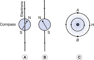
Figure 9.1 (A and B) The effect of the magnetic field produced by the electrons flowing in the wire upon a magnetic compass. (C) If we look along the wire in the direction of electron flow, then the field is an anticlockwise direction (⊗ means that the electrons are flowing away from the eye of the observer).

If the wire is aligned in a north–south direction (i.e. along the direction of the compass needle), then an electric current through the wire causes deflections of the compass, as shown in Figure 9.1: clockwise when the wire is above the compass (A) and anticlockwise when the wire is below the compass (B). This is only possible if the lines of magnetic force are circular and in an anticlockwise direction when viewed along the same direction as the movement of the flowing electrons. We may therefore use the following convention.

This convention is illustrated in Figure 9.1C, where the symbol ⊗ means that electron flow is away from the eye (and ⊙ is towards the eye). The arrows on the lines of force are in an anticlockwise direction, in accordance with our convention, and give the direction in which a north pole would move if placed in that position. Thus, a weightless north pole would, if released, travel round and round the wire indefinitely in an anticlockwise circle.

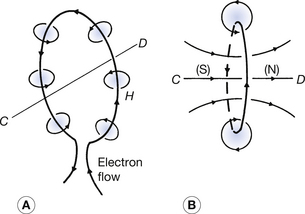
9.5 Magnetic field due to a circular coil of wire

Figure 9.2A shows a circular coil of wire in which an electric current is made to flow. Now, each individual moving electron produces anticlockwise magnetic lines of force about itself, as illustrated in Figure 9.2A. The closeness of the lines of force to each other represents the total magnetic effect (i.e. the magnetic flux density, as described in Sect. 8.2). The addition at a point of all the magnetic flux densities represented by the lines of force produces the total magnetic flux density at that point. Note that, within the coil, the lines of force all tend to be in the direction C to D, while outside the coil, they are from D to C. A top view of the coil (Fig. 9.2B) shows the pattern of the overall lines of force so obtained. It is interesting to note the similarity of these lines of force to those of a short bar magnet (see Fig. 8.1), where they emerge from the north pole end and travel around the magnet to the south pole end and back again. Here we have the reason for the ‘atomic magnets’, where (on a tiny scale) the coil would be equivalent to the net flow of electrons around a particular atomic nucleus, producing lines of force as in Figure 9.2B and hence the magnetized atom.

Figure 9.2 The magnetic field around a coil of wire carrying a current. Note the similarity to the field around a small bar magnet.

9.6 Magnetic field due to a solenoid

A solenoid consists of several coils joined together, and so produces magnetic lines of force, as shown in Figure 9.3A, similar to a bar magnet.

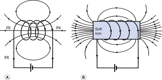
Figure 9.3 (A) The magnetic field produced by a current-carrying solenoid. (B) The large increase in the magnetic field produced when using a soft iron bore in the solenoid.

The effect of a piece of soft iron within the solenoid is to increase the magnetic flux density many times because of the induced magnetism within the soft iron. This effect is reflected by an increase in the number of lines of force in Figure 9.3B compared to Figure 9.3A. The combination of solenoid and soft iron in this manner is known as an electromagnet. The coils in an AC transformer act as a solenoid inducing a magmatic flux in the core of the transformer.

Insight

A general method of calculating the magnetic flux from any general shape of current-carrying conductor is due to Biot and Savart. The formula shown in Figure 9.4 can be used to calculate the magnetic flux density for any general shape of conductor. (Table 9.1 shows some of these examples.)

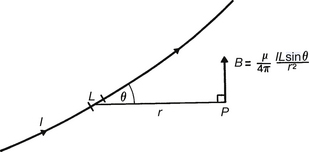
Figure 9.4 Biot and Savart’s law for determining the magnetic flux density due to any shape of current-carrying conductor.(Table 9.1 shows some of these examples)

Table 9.1 Magnetic flux density from different shapes of current-carrying conductors

CONDUCTOR	MAGNETIC FLUX DENSITY, B (TESLA)
Infinite straight wire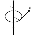
Circular coil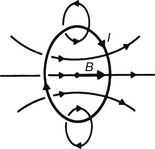
Infinite solenoid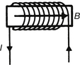	B=μ0l (air only) B=μnl (where n=number of turns/metre)

The effect of aligning atoms is to produce a total flux density, B, within the sample which is greater than that in the air alone, such that:

where μ is the permeability of the medium. Here, the magnetizing force, H, is regarded as the cause of the magnetic flux density, B, in a medium of permeability, μ.

Rearranging the equation in Figure 9.4:

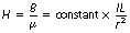
so that the units of the magnetic field strength (or magnetizing force) H are in amperes per metre.