1 Principles of Drug Therapy
The intent of drug therapy is to induce a desired pharmacologic response for a sufficiently long period of time while preventing adverse drug events (see Chapter 4). For most drugs the magnitude of pharmacologic response is proportionately related to the (log of) drug concentration at the tissue (receptor) site (Figure 1-1). Understanding the relationship among dose, drug concentration, and response requires an understanding of the pharmacodynamics (i.e., the science of drug action), or the physiologic and biochemical effects of a drug and their relationship to the drug’s mechanism of actions. Most commonly, the response is measured in the animal but may also occur in a microbe or parasite.1 Pharmacodynamics may be studied in vitro (isolated cells or tissue), ex vivo (isolated cells or tissues after exposure to the drug in the intact animal), or in vivo (exposure and study occurs in the whole animal). Pharmacodynamics ultimately should be integrated with the science of pharmacokinetics, that is drug movements through the body.
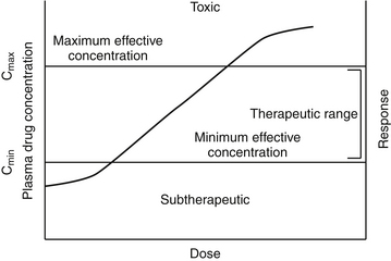
Figure 1-1 The relationship among log plasma or tissue drug concentration and dose and response generally can be considered linear within the concentrations used therapeutically. Ideally, plasma drug concentration will fall within the therapeutic range (between Cmax and Cmin) throughout most of the dosing interval. A representative concentration versus response curve generally yields a sigmoidal shape. At lower (20% response) and higher concentrations (>80% response), larger dose increases are required to stimulate a response. Therapeutic doses should target the linear portion of the curve, between 20% and 80% of the maximal effect. Above that point increasingly larger doses again are needed to generate a change in response, and the risk of toxicity increases, although the dosing interval may be prolonged for safe drugs.
Dose–Response Relationship
Pharmacodynamic responses occur at many levels, ranging from single molecules to whole animals. Drugs induce their responses through a number of mechanisms, most of which involve direct or indirect interactions with cell macromolecules and generally proteins. Direct interactions with nonprotein molecules are less common, but examples include nucleic acids (e.g., cancer chemotherapeutic agents), metal chelating drugs, or antacids used to chemically neutralize gastric acid. Drug responses more commonly reflect the interaction of the drug, acting as a ligand, with receptors (Figure 1-2). A receptor most commonly is a large protein macromolecule (e.g., structural, enzymatic, carrier, or ion channel proteins) responsible for cellular signaling. Receptors may be located on or in the cell membrane, in the cytosol, or within an intracellular structure (i.e., nucleus). Physiologic functions of the body generally are regulated by multiple receptor-mediated mechanisms, each responding to different molecular stimuli. Examples of target receptor categories include hormones, neuromodulatory receptors, and neurotransmitters.
Interaction between a drug and its receptor generally results in activation (either directly or indirectly) of cellular biochemical processes (e.g., ion conductance, protein phosphorylation, or DNA transcription) by way of a transduction pathway that ultimately brings about the pharmacologic effect.1 A time lag may be associated with transduction (Figure 1-2). Activation reflects the drug’s mechanism of action, whereas the sequelae of the stimulation at the molecular, cellular, or tissue level reflect the drug’s pharmacodynamic effects. Secondary intracellular messenger molecules are often activated by drug–receptor interaction; they subsequently set in motion a cascade of events that eventually causes the response. Among the most common receptors are transmembrane receptors linked to guanosine triphosphate–binding proteins (G proteins). These then activate second messenger systems such as adenylyl cyclase (e.g., beta-adrenoceptors), the cytosolic inositol triphosphate pathway (e.g., alpha-adrenoceptors), or membrane-bound diacylglycerol (DAG).
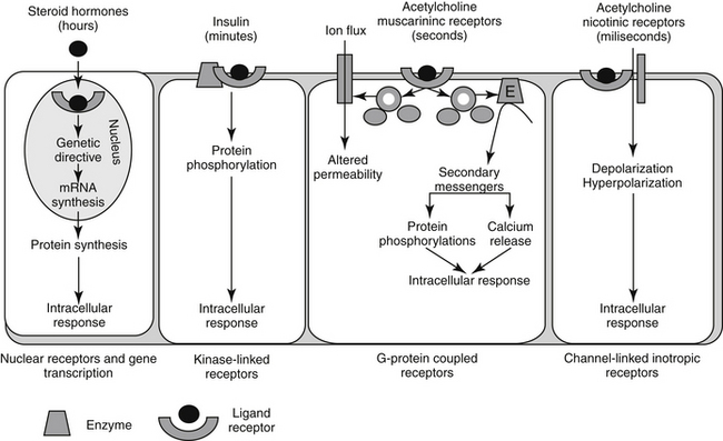
Figure 1-2 Examples of drug–receptor interactions at the cell membrane, cytosol or organelle site, and the secondary amplification cascades that ultimately result in the pharmacodynamic response.
Two properties describe drug-receptor interactions: affinity, or the capacity of a drug to bind to a receptor, and intrinsic efficacy (or activity), or the capacity of a drug to activate or inactivate a receptor. The latter is a complex relationship dependent on drug concentration, receptor activation, and cellular response. Affinity is usually mathematically defined as the reciprocal of the dissociation constant of the drug for the receptor.1 A receptor often is characterized by multiple types (e.g., alpha- and beta-adrenergics; mu, kappa, and delta opioid receptors) and subtypes (e.g., alpha 1 and 2, beta 1, 2, or 3; mu 1 or 2). The selectivity of a drug action generally reflects the specificity of the drug for the target receptor binding. Drugs often target multiple receptors, although interactions may be concentration dependent or may result in blocking rather than activating specific receptors. Receptor characteristics (e.g., numbers and affinities) are influenced by both external and intracellular conditions. Tissues vary in receptor numbers and subtypes; indeed, proper physiologic responses are dependent on this variability. The relationship between a drug and pharmacologic response was at one time assumed to be directly proportional to the number of receptors occupied by the drug, with a maximal response reflecting 100% occupancy and activation (i.e., the drug receptor theory). However, the interactions are much more complex than that described by a simple linear relationship. Different kinetic relationships (linear, log-linear, polynomial), multiple activation states, (active, inactive, resting), cell amplification of the drug-receptor signal, and existence of spare receptors are some examples of the complexities that determine the relationship between drug concentration and response. The scientific description, examination, and ultimate prediction of drug–receptor interactions are often accomplished by generation of dose–response curves; the graphic representation most generally is represented by a sigmoidal curve (Figure 1-3; see also Fig. 1-1). The curve indicates that increasing drug concentration at the receptor site increases the number of bound receptors and thus drug effect. If concentration–response curves are plotted on a logarithmic (x) axis, the portion of the curve that lies between 20% and 80% of the maximal response is generally linear. This is the portion most relevant to therapeutic concentrations and thus encompasses the therapeutic range. Increasing a drug dose within this range generally results in a proportional increase in response. However, once the 80% mark is passed, as receptors become saturated, a much larger increase in concentration (dose) is necessary to increase response. Although this may increase the risk of adverse effects, for drugs which are safe, it may also prolong the dosing interval since the response will not change much as concentrations decline to the 80% level. At that point, drug concentration declines exponentially (generally first order), and response will also decline log-linearly with time (e.g., 50% decline with one half-life). Note that for some drugs (i.e., drugs that irreversibly interact with receptors, drugs with active metabolites,), response may not be related to plasma (tissue) drug concentrations.
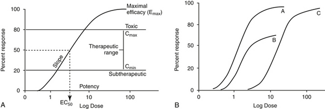
Figure 1-3 Drugs that are equally effective will cause the maximum response but may not be equally potent, i.e., they may not have the same relationship between dose (concentration) and response (A). Because drugs A and C result in the same maximum response (Emax), they are equally effective, whereas drug B is less effective (B). However, drug B is more potent than drug C, and drug A is more potent than both because the dose or concentration of A necessary to achieve a 50% maximum response (ED50 or EC50) is less than that for B or C. A similar set of curves can be used to describe competitive and noncompetitive inhibition. A drug that noncompetitively inhibits another drug will prevent it from reaching its maximum effect, and thus decrease the Emax (plot B, with noncompetitive drug present, plot A without it). In contrast, a drug that competitively inhibits another drug will not alter its Emax, but will increase the concentration of the drug necessary to achieve it (plot C represents a drug with a competitor present; plot A, drug without competitor).
The interaction of a drug with a receptor is similar to that between a substrate binding to the active site of an enzyme. As such, similar equations and parameters are used to describe the relationship between dose and response. The effective dose (ED) is the quantity of administered drug that will produce the (desired) effects for which it is administered. The median effective dose (ED50) is the dose that produces the desired effect in 50% of a population. However, dose is a less accurate descriptor of what is happening at the receptor than is effective concentration (EC). The affinity of the drug for the receptor is described by the (effective concentration) EC50, the drug concentration that yields 50% of the maximal response (see Figure 1-3, A). The different actions of a drug, such as therapeutic and adverse effects, are often due to the drug binding to different receptors with different EC50 values. Ideally, the EC50 for an adverse event is higher than that of a therapeutic response. The ratio of adverse event EC50 to the therapeutic effect EC50 is the therapeutic index and provides some indication of drug safety in that the larger the index, the safer the drug. Efficacy and potency are two terms used to describe the relationship among drug, concentration, and response. Efficacy refers to the maximum effect (Emax) a drug can have (e = 1 indicates a full response), whereas potency is a comparative term that describes the concentration of two drugs necessary to induce the same magnitude of response. Generally, plots describing efficacy and potency are based on log 10 concentration versus percent response curve. (see Figure1-3, A). Drugs are considered equal in efficacy if they can cause the same magnitude of response; the more potent drug will cause an EC50 at a lower concentration. As such, the dose of a less potent drug may simply need to be increased to achieve the same effect of the more potent drug.
Drug–receptor interactions do not always yield the maximal response. Receptor interaction with a drug that acts as an agonist (generally, a structural analog of the targeted receptor) results in some level of activation. The occupation theory of drug–receptor interaction indicates that the magnitude of the response produced by an agonist is directly proportional to the number of receptors occupied.1 Pharmacodynamic antagonism occurs when one drug inhibits the agonistic effects of another through actions at the same pathway, although this does not have to occur at the receptor. Like an agonist, an antagonist interacts selectively with receptors, but it lacks intrinsic efficacy and thus is able to block or reduce the action of an agonist at the receptor. Drugs that target opioid receptors (at least three types, with mu receptors having at least two subtypes) offer an example of the different sequelae of drug–receptor interactions. The “full” agonist (e.g., fentanyl) results in the maximal effect (e.g., at mu receptors). A drug that acts as a “reversal” agent would reduce the effect of an exogenous agonist (e.g., naloxone reverses the effects of fentanyl) whereas a “blocking” drug antagonizes endogenous agonists (e.g., catecholamines targeted by beta- or alpha-blockers). Drugs might have dual agonist and antagonist properties at the same receptor (although to variable degrees in different tissues). Because the response is not maximal, they are referred to as partial (low-efficacy) agonists; buprenorphine is a partial agonist opioid at mu receptors. Drugs might also act as an agonist at some receptors and an antagonist at other receptors. Butorphanol is a mixed agonist/antagonist (at kappa and mu receptors, respectively).
The relationship between an antagonist and receptor can be described as competitive or noncompetitive. Competition between compounds occurs at the same receptors and can be reversible or irreversible. Reversible antagonists easily dissociate from the receptor, whereas irreversible antagonists form a stable chemical bond with the receptor (e.g., in alkylation). If the interaction is reversible, an agonist present at sufficiently high concentrations can displace an antagonist. As such, reversal of the agonist or the response may require a higher dose (or a repeat dose) of the antagonist (see Figure 1-3, B). In contrast, an irreversible antagonist cannot be displaced from the receptor. As such, the cellular response can not occur until the receptor is replaced (duration dependent on rate of receptor turnover) and any remaining unbound antagonist has been removed from the body. The presence of a reversible competitive inhibitor will decrease the potency of a drug because a higher concentration will be necessary to induce the same pharmacologic response.
In contrast, the presence of an irreversible competitive inhibitor will decrease the efficacy of the drug by preventing the maximal possible response. In contrast to competitive antagonists, noncompetitive antagonists interact with receptors at a site different from the agonist–receptor interaction site. The interaction often involves a site in the transduction pathway between the receptor and the pharmacodynamic response.1 Noncompetitive interactions are generally, but not always, reversible. Note that three other types of antagonism, in addition to pharmacodynamic, can occur between drugs: chemical antagonism results from a direct chemical interaction between two drugs (i.e., a weak acid and weak base), physiologic antagonism occurs when two drugs act in the same physiologic system but act on different receptors or pathways, and pharmacokinetic antagonism occurs when one drug alters the response to another drug through changes in disposition (see Chapter 2).
Pharmacodynamic responses are also influenced by the presence of drugs beyond activation. Receptor upregulation and downregulation is an adaptive mechanism that may affect clinical response. Sequelae may include but are not limited to tachyphylaxis, a rapidly decreasing response to a drug after administration of only a few doses; tolerance, a decreasing response to repeated constant doses of a drug that will necessitate a concentration and thus dose increase, if the response is to be maintained; and withdrawal, the syndrome of often painful physical and psychological symptoms that occurs when an addictive substance is discontinued.
The pharmacodynamic response to a drug ideally will occur with any given dose within a therapeutic range. The therapeutic range provides a target for the dosing regimen. It consists of a minimum effective plasma drug concentration (PDC) (trough or Cmin), below which therapeutic failure is likely to occur, and a maximum effective PDC (peak or Cmax), above which a type A adverse reaction (see Chapter 4) is more likely to occur (see Figures 1-1 and 1-3).2,3 Dosing regimens are composed of a dose (e.g., mg/kg) and an interval (e.g., every 8 hours) for each route. The dose of the regimen generally is designed to achieve and maintain PDC within the therapeutic range throughout most of the dosing interval. Thus targeted peak PDCs often approximate but do not exceed Cmax, whereas trough concentrations approximate but generally do not drop below Cmin. However, a therapeutic range is a population statistic that describes the concentrations between which most animals will exhibit the (desired) pharmacodynamic response; each animal will respond (therapeutically or adversely) at a different point in the range. Although most animals will respond at some point within the range (the majority in the middle of the range), a small percentage will respond above or below the range. Therapeutic drug monitoring (see Chapter 5) is used to establish where in the therapeutic range the individual animal will respond; in other words, it will establish the patient’s therapeutic range. Ideally, studies that determine the dosing regimen in a target species reflect integration of pharmacokinetic and pharmacodynamic studies in that species.4 Two primary components of a dosing regimen are dose interval. In general, dose, which ultimately determines PDC, is influenced primarily by the tissue that dilutes the drug (i.e., volume of distribution), whereas interval is influenced by elimination of the drug (i.e., half-life). Unfortunately, studies that describe the time course of a drug in animals are limited and, when available, generally focus on healthy rather than diseased animals. As such, clinicians are faced with individualizing dosing regimens in the patient according to the principles of clinical pharmacology—that is, the study of drugs5 and their behavior (disposition)6 in animals.
Determinants of Drug Disposition
Mechanisms of Drug Movement
Drugs move through the body by two major mechanisms: bulk flow and passive diffusion. The cardiovascular system is the primary determinant of bulk flow; glomerular filtration is one of the more important specific examples. The chemical nature of the drug does not affect bulk flow. Most drugs are characterized by a molecular weight (MW) of 350 or less, ensuring movement of unbound drug between endothelial cells despite the presence of protein filters in the endothelial gaps. Exceptions are made for those tissues whose capillaries are not fenestrated, because endothelial cell junctions are tight. Drug movement for these tissues must occur across cell membranes. Drugs can move through cells directly through the lipid layers of the cell (e.g., passive diffusion), through aqueous pores formed by aquaporins (proteins) that span the width of the membrane, by combination with transmembrane carrier proteins, and by pinocytosis. Of these, transmembrane (passive) diffusion and carrier-mediated movement are most important.
KEY POINT 1-1
Passive diffusion is the most common method by which compounds move through the body. It is most influenced by the concentration gradient of diffusible drug across the membrane to be diffused.
Passive diffusion occurs independent of any other mechanism of drug movement and requires no energy. Passive diffusion through cell membranes depends on a number of factors. The single most important factor is concentration of diffusible drug, which is most easily manipulated by increasing the dose. Additionally, host and drug factors will also influence the concentration of diffusible drug. Host determinants of passive diffusion are subject to change and include thickness of the membrane to be traversed (inversely proportional; e.g., edematous compared with normal tissues), surface area (directly proportional; e.g., small intestine versus stomach), environmental pH (see ionization), and temperature (directly proportional). In contrast, drug characteristics influencing passive diffusion are not subject to change, and thus cannot be easily manipulated. They largely influence lipid solubility of the drug.2,3 Lipid solubility is, in turn, influenced by a number of drug characteristics, including the inherent chemical structure of a drug, such as molecular weight (smaller molecules diffuse more easily) and partition coefficient (PC). The PC is an experimental measure of relative lipid solubility as influenced by the chemical structure of the drug. The ratio is determined by mixing the drug in a combination of water and an organic solvent (e.g., octanyl). The difference in drug concentration between the two solvents once mixing is complete reflects, in part, the inherent lipid versus water solubility of the drug. Measurement of the concentration of drug in each solvent generates an octanyl:water coefficient or PC, which might be useful for predicting the ability of a drug to pass through cell membranes. A ratio greater than 1 suggests greater distribution to the organic phase, indicating lipid solubility. For example, in regards to providing analgesia, fentanyl (PC of 717) is both more potent and more rapid acting, but shorter in duration, compared to morphine (PC of 0.7), presumably because it can move more rapidly through the blood–brain barrier (Figure 1-4). Benzene rings, carbon double bonds and methyl groups tend to make a drug more lipid soluble, whereas polar compounds such as amine or hydroxyl groups contribute to drug-water solubility.
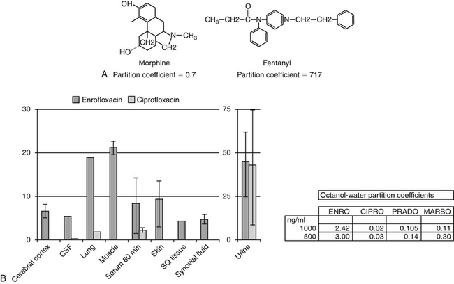
Figure 1-4 Lipid solubility of a compound can be predicted on the basis of the octanyl: water partition coefficient (PC), which in turn depends on chemical structure. A, Morphine and fentanyl both reach the central nervous system in sufficient quantity to provide analgesia. However, fentanyl is much more lipid soluble, as is supported by its octanyl:water partition coefficient of 717 compared with that of morphine (0.7). Fentanyl is much more potent and more rapid acting, but it also has a shorter duration of effect. B, The PC among the fluorinated quinolones suggests that enrofloxacin would have better tissue distribution than ciprofloxacin. This is supported by the relative concentrations of enrofloxacin versus ciprofloxacin in serum compared with tissues 60 minutes after administration of 20 mg/kg intravenous enrofloxacin in dogs. Although PC is an important determinant of lipid solubility, it may vary with surrounding pH. (ENRO, enrofloxacin; CIPRO, ciprofloxacin; PRADO, pradofloxacin; MARBO, marbofloxacin.)
KEY POINT 1-2
A drug will be more nonionized and more likely to diffuse into tissues when present in a “like” environment—that is, acidic drugs in an acidic environment.
In addition to lipid solubility, drug pKa and environmental (host) pH will also influence distribution of drug into body compartments. The Henderson-Hasselbalch equation describes the pH partition theory (Figure 1-5). Assuming a drug is sufficiently lipid soluble to cross cell membranes, a steady-state equilibrium will be reached when the amount of drug moving from one area equals the amount moving in the opposite direction and the concentration of diffusible drug will be equivalent on either side of a membrane. However, in its ionized form, a drug is not diffusible, cannot traverse lipid membranes, and becomes trapped and thus “partitioned” by the pH in its surrounding environment. Although the concentration of the nonionized (diffusible) portion on each side of the membrane will be equal (assuming a steady state equilibrium is reached), the total concentration on either side may differ if the pH on either side of the membrane is different (Figure 1-5). The difference depends on the pKa of the drug and the environmental pH on either side of the membrane. Drugs will be trapped by ionization when present in an “unlike” environment. Drug pKa (the pH at which the drug is 50% ionized and 50% nonionized; ratio 1:1), and its behavior as a weak acid or base defines the degree of ionization. For a weak acid, as local pH decreases (becoming more “like”), the nonionized and thus diffusible proportion will increase. In contrast, for a weak acid, an increase in pH (“unlike”) will increase the ionized proportion. The opposite is true for a weak base: increasing pH will increase the nonionized or diffusible proportion, whereas a pH decrease will increase the ionized, nondiffusible portion (Box 1-1).
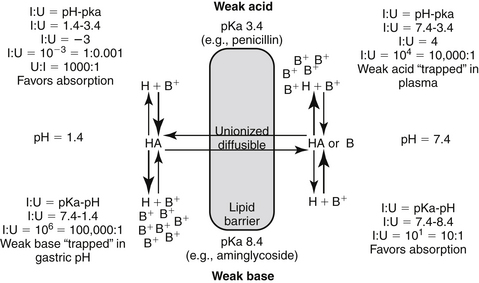
Figure 1-5 The Henderson-Hasselbalch equation and the pH partition hypothesis predict the behavior of an ionizable compound on the basis of its pKa and the ambient pH. A weak base (bottom) will be predominantly ionized in an acidic environment (i.e., gastric pH), and thus is likely to be trapped. It is less likely to be ionized in a higher pH and thus is more diffusible (i.e., plasma). In contrast, a weak acid (top) is likely to be nonionized in the acidic environment and thus is more likely than the weak base to move across the lipid membrane and be absorbed. However, in the plasma the higher pH will increase the proportion of ionized drug, limiting its diffusion from plasma into cells. (see Box 1-1.)
Box 1-1 The pH Partition Hypothesis
The pH partition hypothesis is the ratio of ionized:nonionized drug and is based on pH (of the environment) and pKa (of the drug) (see Figure 1-5). The proportion of ionized to unionized drug is described by the Henderson-Hasselbalch equation. For acids, the ratio (ionized:nonionized) is 10n, and for a weak base the ratio is 10-n. The ratio of the ionized:nonionized (I:U) drug can be useful for predicting movement between tissues. A drug is considered significantly ionized if the ratio (I:U) is greater than 100. Thus for a weak acid the drug is considered ionized in an environmental pH that is 2 or more higher than its pKa (pH − pKa = 2; 10n = 102 = 100 I : 1 U) A weak base is considered ionized if the pH is or 2 or more below its pKa.. (pH − pKa = -2; 10-n = 10-(-2) = 102 = 100). Ideally, for drug movement to occur by passive diffusion, the pH will be no more than 2 pH units above the pKa for the acid and no more than 2 pH units below the pKa for the base. The gastrointestinal tract (pH 6.0) offers an example of how pH partition influences drug movement. Orally administered aminoglycosides (weak bases with pKa approximating 7 to 9) are ionized at a ratio of approximately 1000:1 (6 − 9 = −3, 10 -n = 10 –(-3), = 103 = 1000:1 [I:U]. Thus there is only one nonionized or diffusible ion for each 1000 ionized amikacin molecules. The ionized molecules will be trapped and will not be absorbed, limiting absorption of this water-soluble drug. In contrast, the proportion of the ionized weak acid penicillin (pKa about 2) would be 0.0001:1 (2 − 6=10-4); for every ionized molecule, 10,000 molecules would be nonionized (the inverse of 0.0001:1). As such, if other factors are supportive (e.g., the drug is not destroyed by the gastric acidity), penicillin should be well absorbed from the gastrointestinal tract. The urine is another site where pH partition may influence drug movement. Penicillin located in urine with a pH of 7 would be ionized at a ratio of 10,000:1 (105), whereas the aminoglycoside would be ionized at a ratio of only 100:1. If the urine pH was 8, the ratio of I:U would be 10 for the aminoglycoside, which is not considered significant to preclude drug movement. In either pH the aminoglycoside would be more likely than the penicillin to be passively resorbed and to penetrate microbial membranes. Drug that is partitioned by ionization acts as a reservoir, replacing nonionized drug that may leave the other side of the membrane in an open system. Eventually, assuming the nonionized side remains “open,” both sides of the membrane will eventually be depleted of drug.
Although less common, drug movements other than passive diffusion and bulk flow influence PDC. Carrier-mediated transport includes both facilitated diffusion (nonactive) or active transport. An example important transport system is the P-glycoprotein system, an MDR-1 gene product best known for imparting multidrug resistance to cancer cells (and to microbes).7 However, this transport system occurs in several tissues in the body, including renal tubular brush borders and bile canniculi (responsible for drug excretion from the body); the brain or other “sanctuaries” (responsible for keeping exogenous componds out of critical tissues); characterized by a blood–tissue barrier; and in portals of entry, including the lower gastrointestinal tract (reducing oral drug bioavailability).8 Pinocytosis is a rare drug movement exemplified by the uptake of vitamin B12 in the ileum and aminoglycosides by renal tubular cells.
Plasma Drug Concentrations
Although response to a drug reflects concentrations at the tissue (or cellular level), because tissue samples cannot be collected easily, drug concentrations at the tissue site are approximated by measuring PDCs. After administration of a fixed dose of a drug, several drug movements act in concert to determine PDC (Figure 1-6).2,3,6,9 These movements largely, but not exclusively, depend on passive diffusion of the drug and include absorption (A) from the site of administration to systemic circulation, defined as the major vessels and well-perfused organs; distribution (D) of the drug from systemic circulation to tissues (target and nontarget) and back again; and elimination of the drug from the body by metabolism (M) and excretion (E). These drug movements are dynamic, occurring simultaneously, and their net effects determine PDC at any time during the dosing interval after administration of a fixed dose. Because passive diffusion is the major determinant of each drug movement, each in turn is influenced by a number of other factors. The impact of these factors on the drug movements and the time course of drug in the body as a result of these movements can be described or modeled mathematically, leading to the study of pharmacokinetics. Each drug movement is influenced by host and drug factors that may affect therapeutic success (see Chapter 2).
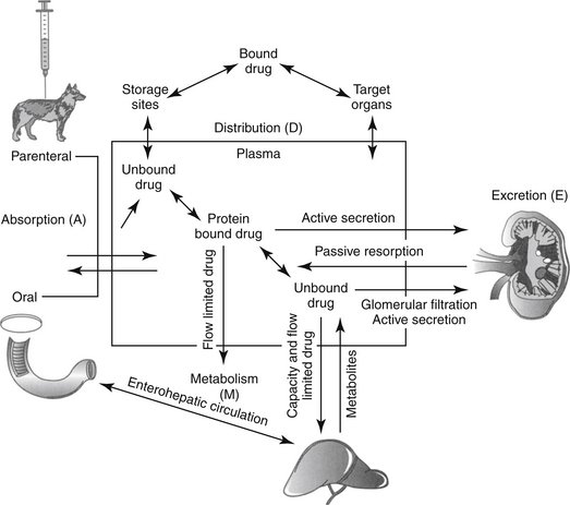
Figure 1-6 The determinants of plasma drug concentration (ADME) act in concert after administration of a fixed dose. The drug must first be absorbed, most commonly from the gastrointestinal tract (Absorption–A). Orally administered drug passes through the liver before reaching systemic circulation (not shown). Once in circulation, drug not bound to plasma proteins (free drug) is distributed into tissues (Distribution–D), where it can be bound to tissues or distributed back to circulation. Elimination of the drug from the body occurs by hepatic metabolism (Metabolism–M) and renal or biliary excretion (Excretion—E) of the drug or its metabolites. Drugs that are protein bound will not be filtered by the kidney or metabolized by the liver unless actively secreted in the kidneys and or characterized by flow-limitation in the liver. Excreted drugs can be passively reabsorbed by the kidney or following biliary excretion after deconjugation in the gastrointestinal drug (enterohepatic circulation).
(Adapted from Ettinger SJ, Feldman EF, editors: Textbook of veterinary internal medicine, ed 5, Philadelphia, 2000, Saunders.)
KEY POINT 1-3
Plasma drug concentrations at any point in time after administration of a dose reflect the combined effects of four dynamic drug movements: absorption, distribution, metabolism, and excretion.
Absorption
Bioavailability, extent, and rate of absorption
The percentage of an administered dose of drug that reaches systemic circulation and is thus able to induce a response is referred to as bioavailability (F).2,3,9,10 Bioavailability (see Pharmacokinetics section) is used to predict drug efficacy after different routes of administration or administration of different formulations of the same drug. Absolute bioavailability or extent of absorption is the actual bioavailability and can be determined only by comparing the appearance of the drug preparation to that after intravenous administration of the drug. In contrast, relative bioavailability of two different preparations or by two routes of administration of the same drug can be evaluated by comparing their area under the curve (AUC).10 The area under the concentration versus time curve (AUC) describes the entire time course of the drug. Because its magnitude depends on maximum drug concentration and rate of elimination, it is influenced by several drug movements, including absorption. The AUC is used to calculate several other pharmacokinetic parameters; clinically, it is useful for determining response to certain drugs, particularly antimicrobials.11,12
KEY POINT 1-4
Absolute bioavailability of a drug preparation can be determined only by comparing its appearance to 100% availability, which occurs only after intravenous administration.
The greater the bioavailability, or extent of absorption of a drug, the greater the anticipated pharmacologic response. However, pharmacologic response of two different drug preparations or the same drug given by different routes may vary even if equally bioavailable; two products are considered bioequivalent only if neither their rate nor their extent of absorption differ. Differences in the rate of absorption (e.g., absorption half-life [see Pharmacokinetics section]) may cause different time to onset, as well as lower peak concentrations, although the duration of effect may be longer.
Factors impacting drug absorption are most profound for orally administered drugs. Factors impacting other routes are addressed under “Routes of Administration.”
Oral absorption
Most orally administered drugs reach systemic circulation after absorption from the small intestine. The rate and extent of drug absorption in the gastrointestinal tract depend on a number of host factors, most of which affect passive diffusion (Figure 1-7).9 These include gastrointestinal pH, which favors absorption of weak acids; surface area, which favors absorption in the small intestine compared with the stomach; motility, which mixes the drug, the concentration of diffusible drug at the site of movement; permeability and thickness of the mucosal epithelium; and intestinal blood flow, which maintains the concentration gradient across the mucosal epithelium. The latter factor of blood flow is important only for drugs capable of rapid transfer across the epithelium.
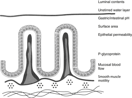
Figure 1-7 The determinants of oral drug absorption include local pH, the surface area to which the dissolved drug is presented, epithelial permeability, mucosal blood flow (particularly for drugs very rapidly absorbed), and smooth muscle motility. The drug must be diffusible, and thus must be in the dissolved state (to establish a concentration gradient). Most drugs are absorbed in the small intestine because of its larger surface area. The drug transport system, P-glycoprotein, decreases bioavailability through drug efflux from the intestinal epithelial cell.
In general, the intestinal surface area is so large that changes seldom are of sufficient magnitude to effect absorption (see Chapter 2). However, changing particle size of the drug preparation may cause differences in the rate or extent of absorption and markedly different bioequivalences. Drug preparations often are specifically designed to alter rates of absorption by manipulation of particle size.
Bioavailability of an orally administered drug also is influenced by factors after it passes into the gastrointestinal epithelium. Bioavailability is decreased if the drug is metabolized by intestinal epithelial cells, microbes, or by the liver. Additionally, enterocytes can decrease oral bioavailability of a drug by causing its efflux from enterocytes, in part because of the presence of active transport proteins located on enterocyte cell membranes.13
Transport membranes may act alone or in concert with one another; for some drugs, one transporter may predominate, but for others, none may. Identifying the role of each transporter protein is complicated and difficult to study. Several families have been identified. (1) Transporters located on the apical cell membrane include the family of organic anion-transporting polypeptides (OATPs); these proteins are also located in the liver, kidney, and brain and influence distribution and excretion. These proteins transport a large number of amphipathic drugs (e.g., digoxin, steroids) and endogenous compounds (e.g., steroids, thyroid hormones). (2) Proton-dependent oligopeptide transporters (POTs), driven by a proton gradient, are present in the kidney, brain, and the gastrointestinal tract, where their activity appears to increase from the duodenum to the ileum. Among the drugs influenced by these transporters are beta-lactam antimicrobials, ACE-inhibitors, and prodrugs of selected antivirals. (3) The family of ATP-binding cassette (ABC) superfamily of transporters includes the P-glycoproteins. These include multidrug resistance protein (MRP1) and a multispecific organic anion transporter (MOAT) also located in other tissues. An efflux transporter, P-glycoprotein is characterized by broad substrate specificity. Because it is abundant in enterocytes, it can profoundly decrease the oral bioavailability of target drugs. It is associated and shares substrate specificity with selected cytochrome-P450 enzymes (most notably, CYP3A), which decreases drug that is not effluxed from the cell by the transporter (see Chapter 2).13
Hepatic metabolism also can profoundly affect the PDC of an orally administered drug. After gastrointestinal absorption, drugs enter the portal vein and then the liver (Figure 1-8). As such, an orally administered drug is exposed to hepatocytes before it enters the systemic circulation. Drugs characterized by a high hepatic extraction ratio (>70% extracted) are almost completely removed from the blood by hepatocytes during the first passage of blood through the liver. As a result, after oral administration, drugs that undergo first-pass metabolism may not reach systemic circulation in concentrations sufficiently high to cause a pharmacologic response. Despite good to excellent oral absorption, such drugs are characterized by poor bioavailability and are administered either parenterally (e.g., lidocaine) or in oral doses high enough to compensate for first-pass metabolism by the liver. Examples of drugs that are orally administered yet undergo significant hepatic first-pass metabolism include selected cardiac drugs (e.g., propranolol and other beta-blockers, diltiazem in some species, hydralazine, nitroglycerin), diazepam, and opioid analgesics. The negative effects of first-pass metabolism on pharmacologic response may be reduced if the drug metabolites (e.g., propranolol and diazepam) are also pharmacologically active.
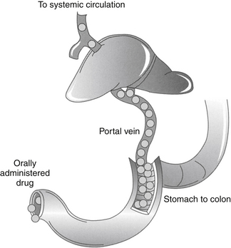
Figure 1-8 First-pass metabolism occurs as drug absorbed from the gastrointestinal tract (from the stomach to the lower colon) enters the portal vein and flows to the liver. Once in the liver, drugs that are characterized by a high extraction are removed rapidly from the blood before entering systemic circulation. Plasma concentrations of such drugs may not reach therapeutic concentrations unless the dose is increased to compensate for first-pass metabolism. The amount of drug removed on the first pass from the liver differs among species and ages and according to the presence or absence of disease. First-pass metabolism can be avoided by transmucosal absorption in the oral cavity, or rectal absorption,
Distribution
Once a drug reaches the systemic circulation, it must be distributed from the central (blood) compartment to peripheral tissues to impart a pharmacologic effect. Further, drug in tissues will be distributed back into plasma so that it can be eliminated. The major factors that determine drug distribution to and from tissues include drug lipid solubility and its ability to penetrate cell membranes, the degree to which the drug is bound to plasma or tissue proteins, and regional (organ) blood flow. The presence of transport proteins (p-glycoprotein, OATPs, and POTs) also influence drug distribution, particularly in “sanctuary” tissues characterized by tissue–blood barriers (e.g., brain, cerebrospinal fluid, placenta).13
Binding of lipid-soluble drugs to plasma proteins facilitates their circulation. Drug binding to proteins may influence several determinants of drug movement, including distribution.14 Weakly acidic drugs tend to bind to albumin, whereas weakly basic drugs tend to bind to α1‑glycoproteins.15 The large molecular weight of protein precludes movement of bound drug from circulation into tissues. As such, the protein-bound drug is not pharmacologically active; cannot be filtered in the normal glomerulus, and for some drugs (i.e., capacity-limited, discussed later), cannot reach drug metabolizing enzymes in the hepatocyte (or other organ). Presumably, drugs that are highly protein bound may be more likely to be involved in adverse reactions early in the dosing regimen because displacement of only a small proportion of drug from the protein (e.g., due to competition with other protein-bound drugs or hypoalbuminemia) can increase the total amount of free, active drug (Figure 1-9).2,3 A drug is considered significantly (highly) protein bound if 80% or more bound; for a drug bound less than 80%, displacing enough drug to significantly increase the unbound proportion is difficult. For example, displacement of only 1% of a drug that is 99% protein bound (e.g., nonsteroidal antiinflammatories) can double the concentration of pharmacologically active drug. In contrast, to double the pharmacologically active form of a drug that is only 80% bound (i.e., going from 20% to 40% unbound) would require displacement of 25% of the bound drug, which is clinically difficult to achieve. Yet even with highly protein-bound drugs, the clinical relevance of displacement and increased concentrations of unbound drug is questionable: in the face of normal renal and hepatic function, clearance of the freed drug by these organs will increase such that “extra” drug is rapidly removed.16 However, it is not clear that clearance will increase sufficiently in the face of organ dysfunction (e.g., renal or liver disease). Further, the package insert for Converia, which is highly protein bound, indicates that the plasma drug concentration of several other highly protein bound drugs increased with co-administration.
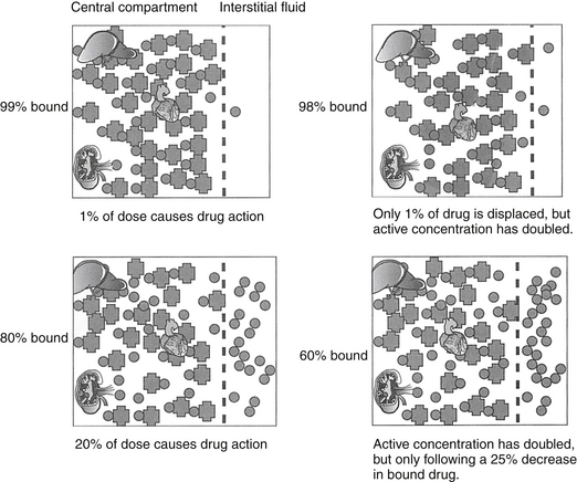
Figure 1-9 Displacement of drug from protein-binding sites becomes significant only if a drug is greater than 80% protein bound. Displacement of only 1% of a drug that is 99% protein bound doubles the pharmacologically active form of the drug (top two diagrams). For a drug that is 80% protein bound, however, 20% of the dose is responsible for pharmacologic actions. Displacement of 25% of the drug is necessary to double the pharmacologically active drug. However, because unbound drug will be cleared more rapidly (assuming normal organ function), displacement of highly bound drugs may not be clinically important.
In addition to its ability to reach target tissues and organs of elimination, distribution of a drug is important because of its influence on PDC and drug elimination. The amount of tissue to which a drug is distributed, often estimated by the theoretical parameter, volume of distribution (Vd) of the drug, directly but inversely influences PDC.2,3,17 Because it is theoretical, Vd is generally referred to as apparent Vd. The Vd of a drug also describes the ease with which the drug leaves the plasma. Simplistically, volume of distribution is also the volume to which a drug would have to be distributed if it were present throughout the body in the same concentration as that measured in the plasma after intravenous (IV) administration of a known dose. It can be exemplified by adding 5 g of dextrose (considered the dose) to each of two beakers containing a different but unknown volume of water. The dextrose is allowed to distribute equally throughout the beaker (no membranes are present in the beaker) and then the concentration is measured. If the concentration in beaker A is 5% (50 mg/mL or 5 g/100 mL), then the volume of water in the beaker must be 100 mL. If the concentration in beaker B is 2.5% (25 mg/mL or 25 g/100 mL), the volume must be 200 mL. The Vd in beaker A is twice that in beaker B. The Vd of a drug in an animal is determined essentially the same way: a known dose is given intravenously to ensure that all the drug reaches the site being measured, the drug is allowed to distribute until equilibrium (or pseudo-equilibrium) is reached, and the peak drug concentration is determined. The Vd is then calculated by dividing the dose by the peak concentration (the y intercept, Co, A or B): Vd = Dose/Co (see the Pharmacokinetics section).
The PDC (and response to) a drug at a known dose varies inversely with Vd. Vd differences among species and ages (pediatric versus geriatric) can dramatically affect PDC (see Chapter 2). In addition, diseases associated with fluid retention or obesity are likely to increase the Vd of many drugs (and thus decrease PDC), whereas dehydration or weight loss is likely to decrease Vd and thus increase PDC (see Chapter 2). The impact depends upon whether the drug is distributed to total body water (i.e., a lipid-soluble drug) or extracellular fluid (i.e., a water-soluble drug). Because the distribution of a drug to peripheral tissues removes drugs from organs of drug clearance, Vd also directly and proportionately influences elimination half-life (Figure 1-10). Thus any factor that increases Vd will tend to decrease PDC but prolong the elimination half-life and thus the presence of the drug in the body.
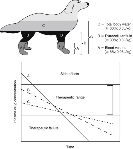
Figure 1-10 Despite its theoretical nature, the size of the apparent volume of distribution (Vd) may indicate the body compartment to which the drug is distributed. These include (A) the blood compartment (i.e., a drug tightly bound to plasma proteins), (B) extracellular fluid (e.g., a water-soluble drug), or (C) total body water (i.e., a liphophilic drug that penetrates cell membranes). Increasingly larger volumes represented by these compartment inversely affect plasma drug concentration (PDC) and the slope of the elimination (kel) curve. This curve determines elimination half-life, which changes directly with Vd.
If a semipermeable membrane divided the beakers used to exemplify Vd into two compartments, distribution of the dextrose throughout each beaker would have taken longer than if the membrane were not present. At distribution equilibrium, (the amount of drug moving from one side equals the amount of drug moving from the other side. Further, at equilibrium, although the amount of drug passing between the two compartments is equal, membrane or fluid characteristics result in different concentrations of drug on each side of the membrane after equilibrium has been reached. Thus both the rate (i.e., distribution half-life) and extent of drug distribution may be affected by membranes. The body contains many membranes whose characteristics are sufficiently complex that multiple compartments may be formed. Extracellular and intracellular compartments (which together make up total body water) are major compartments to which drugs distribute. Most capillaries are fenestrated and present no barrier to passage of unbound drugs from plasma to interstitial fluid. Hence water-soluble drugs tend to be distributed to extracellular fluid (ECF; 20% to 30% of body weight) and thus are often characterized by a Vd of 0.1 to 0.3 L/kg. Lipid-soluble drugs tend to cross cell membranes and thus distribute into both ECF and intracellular fluid (ICF; i.e., total body water [TBW]) and as such, generally have a larger Vd (>0.6 L/kg). The Vd of highly protein-bound drugs reflects the plasma compartment, and as such is very small (0.05% of the body weight, or 0.05 L/kg). Such drugs may appear to distribute to their total volume almost instantaneously, resulting in a PDC versus time described by a single component, or a one compartment model (see the pharmacokinetics section). However, it is the Vd of the unbound or pharmacologically active drug that is more descriptive of the disposition and pharmacologic effects of a highly bound drug.
Capillaries of selected organs, including the brain, cerebrospinal fluid, eye, testis, and prostate, are not fenestrated, and drugs must diffuse through the capillary endothelium to penetrate these tissues.18,19 For treatment of such organs, lipid-soluble drugs (i.e., Vd >0.6 L/kg) are more likely than water-soluble drugs to penetrate the endothelial barrier and achieve therapeutic concentrations. However, simply because a drug has a Vd that equals or exceeds the volume of TBW does not assure lipid solubility nor does it guarantee sufficient tissue distribution. Drug distribution to various tissues differs with drug chemistry, and intracellular accumulation may occur for many reasons. Ion trapping was previously discussed; drugs also can bind to intracellular proteins (i.e., Na+ K+ ATPase of digoxin), bone (e.g., Ca2+ or Mg+ by tetracyclines) or other macromolecules (e.g., lysozymes by aminoglycosides). Bound drug is generally not active (unless binding occurs to target ligands), but bound drug may act as a reservoir for interstitial and plasma drug concentration (e.g., the antimicrobial cefovecin). Ion trapping or binding of a drug will remove it from plasma; as such, as PDC decreases, for any given dose, the Vd will increase. The Vd of a drug characterized by such multicompartments may result in a Vd that is greater than the volume of the animal (e.g., >1 L/kg). Such a drug exemplifies the theoretical nature of Vd in that it simply (mathematically) describes the amount of tissue that is diluting the drug if the concentrations measured in plasma were the same throughout the body. Although Vd is a useful parameter, particularly for calculating drug dose, it should not be used to indicate where (i.e., ECF, ICF, TBW, or selected tissues) a drug has distributed. Further, because the rate and extent of drug distribution to tissues varies, the time to equilibrium also will vary. Calculations for Vd (and determining peak PDC) generally should not occur until distribution equilibrium has been reached.
KEY POINT 1-5
Volume of distribution is used to calculate the dose by estimating the volume of tissue that will dilute the drug after its intravenous administration. It is theoretical because it provides no information regarding the site of distribution. However, it proportionately impacts plasma drug concentration (inversely) and elimination half-life (directly).
The term distribution equilibrium, or steady-state equilibrium, is often used to refer to the state in which the amount of drug leaving plasma for tissues is equivalent to the amount of drug leaving tissues for plasma. The reality is that distribution equilibrium may not ever be achieved because drugs are characterized by an “open” system—that is, drug is continually being eliminated. Hence, the term pseudoequilibrium is more appropriate. Distribution equilibrium is less likely to be achieved for drugs with a short half-life, particularly when administered at a long dosing interval. Drugs that accumulate (given at a dosing interval that is shorter than the half-life; see later discussion) are more likely to reach a state of equilibrium between doses, although the actual concentrations may fluctuate between Cmax and Cmin during a dosing interval.
Documenting the extent to which a drug distributes to a specific site is difficult because techniques are required that allow collection of interstitial versus intracellular tissue. Measurement of drug in interstitial fluid or ICF might confirm the site of drug distribution. However, collecting a sample of sufficient size using methods that are not traumatic (and thus do not impact drug movement) is difficult. Several techniques have been developed to collect fluid representative of ECF. Examples include tissue cage models; “wick” methods; and more recently and perhaps most appropriately, the use of microfiltration systems that collect directly from ECF using a microprobe. A less representative method of reporting tissue concentrations is measurements of drug in homogenized tissues; this measures both extracellular and intracellular drug. Drugs bound (trapped) inside a cell (e.g., as a result of binding to proteins, or ionization) may markedly increase drug concentrations in homogenized tissue, but the drug may not be pharmacologically active or available to interstitial tissues. However, intracellular drug may act as a reservoir, providing continued input to interstitial fluid even as PDCs decline. Drug-void cells, on the other hand, will artificially dilute actual drug concentrations in the ECF.
KEY POINT 1-6
If a protein-bound drug is displaced from its binding protein, the increase in concentration of free and thus active drug is likely to be short-lived as the free drug is cleared more rapidly in the normal animal, thus potentially offsetting any risk associated with increased concentration.
Thiobarbiturates and propofol undergo a phenomenon of redistribution, relevant only for drugs for which an immediate effect can be realized (i.e., general anesthetics). After a rapid intravenous bolus administration of these drugs, they distribute first into a “central blood pool” composed of low-volume, high-blood-flow organs such as the brain. Anesthetic effects occur rapidly. However, the drug effect rapidly terminates, primarily because of redistribution from the brain to lean tissues such as muscle (Figure 1-11). Continued redistribution to fatty tissues further reduces PDC and thus the pharmacologic effect; sight hounds (which lack body fat) tend to have a prolonged recovery with these drugs. The effects of these drugs are also magnified in the presence of hypovolemic shock because a higher percentage of blood containing the drug flows to the brain and heart.
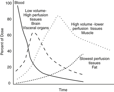
Figure 1-11 The phenomenon of redistribution involves the rapid distribution of drugs to a central blood pool composed of low-volume, high-blood-flow organs such as the brain followed by rapid redistribution to lean tissues. Further redistribution to fatty tissues further reduces plasma drug concentration and thus the pharmacologic effect. Sight hounds tend to have a prolonged recovery with these drugs because redistribution to the fat compartment is less. The effects of these drugs are also magnified in the presence of hypovolemic shock because a higher percentage of blood containing the drug flows to the brain and heart.
Drugs that distribute to TBW may take longer than distribution to ECF. Clinically, peak PDC (Cmax) cannot be assessed until distribution has reached equilibrium (or pseudo-equilibrium). If PDCs are being monitored in a patient, blood samples for peak drug concentrations should not be collected until this time. For orally administered drugs, distribution occurs during absorption and sampling should occur after absorption is complete, generally within 1 to 2 hours after administration.
Metabolism
The rate at which a drug is excreted from the body is the final determinant of PDC. Most drugs are eliminated by hepatic metabolism, renal excretion, or both.2,3 Lipid-soluble drugs require conversion to a water-soluble form before they can be eliminated by the kidney; otherwise, their passive resorption in the renal tubules would preclude excretion. A single change in the molecular structure of a lipid-soluble drug to a more water-soluble form may reduce a half-life of weeks or months to only a few hours. Metabolism can occur in two phases (Figure 1-12). Drugs or their metabolites may undergo both phases or only phase II metabolism. In general, phase I metabolism chemically changes the drug so that it is more water soluble and thus more susceptible to phase II metabolism; phase II metabolism generally renders the drug sufficiently water soluble to be renally excreted. An exception is made for some phase II metabolites (e.g., selected acetylated compounds) that may not only remain reactive but also may be more lipid soluble than the conjugated metabolite.
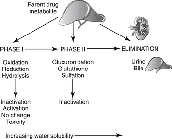
Figure 1-12 Hepatic metabolism can occur in one, two, or multiple phases. Phase I reactions are oxidative, most often accomplished by cytochrome-P450 (hepatic microsomal) enzymes. Phase I metabolites may be subjected to either phase I or phase II metabolism. Although phase I metabolites may be inactivated, they may also be the only active form of the drug (prodrugs). Metabolites may also exhibit similar, less, or more activity compared to the parent compound. Finally, they can also be an important source of drug-induced toxicity. Phase II metabolism generally inactivates the drug. The rate and extent of both phases of metabolism vary among species, ages, and disease states.
KEY POINT 1-7
Perhaps more so than any other factor affecting drug disposition, drug metabolism is complicated by physiologic, pharmacologic, and pathologic factors.
The majority of drug metabolism occurs in the liver. However, the liver is not the only site of drug-metabolizing enzymes; other organs with substantial metabolic capacity attributable to CYP or other enzymes include the kidney and portals of entry (i.e., lungs, skin, and gastrointestinal tract). Most drug-metabolizing enzymes are located in the smooth endoplasmic reticulum (SER) of the hepatocyte; others are located in the cytosol of the cell. Those located in the SER generally consist of a protein (cytochrome) with an iron central core (pigmented like hemoglobin, hence “P”) that, when bound to carbon monoxide, absorbs light at 450 nm; as such, the isozymes are referred to as cytochrome P450 enzymes (CYP450 or simply CYP). When the liver is subjected to homogenization and special centrifugation procedures, the SER forms vesicles or microsomes that contain drug-metabolizing enzymes; hence these enzymes also are referred to as microsomal drug-metabolizing enzymes. These enzymes are actually an enzyme system that can be identified genetically as a superfamily containing several families of enzymes.20-23 Classification and nomenclature of CYP450 is based on gene sequence similarity. The importance of enzymes in humans and the proportion of drugs metabolized by the respective enzyme are 1A2 (13%), 2A6 (4%), 2B6 (1%), 2C (18%), 2D6 (1.5%), 2E1 (7%), and 3A4 (30%). All CYP-mediated drug metabolic reactions involve the addition of a single atom of oxygen onto the substrate; as such the CYP drug-metabolizing system is actually an electron-transport system, and oxygen radicals are generated during the metabolic process. Iron serves as a mechanism for separating molecules of oxygen; a lipid environment, (NADP reductase serves as the electron donor) and oxygen are required for CYP-catalyzed metabolism to occur. Not surprisingly, overlap among drug substrates for the different isozymes is among the reasons that isoenzyme activity can not be predictably extrapolated among species. Inducers and inhibitors differ in normal animals, among species, breeds, ages and gender, as well as tissue. Different concentrations of the various isoenzymes in tissues contribute to tissue specificities of some drug toxicities. The patterns of drug metabolism are complex, and the sequelae of the reactions variable. Drugs can be metabolized through several pathways, and metabolites often are further metabolized; metabolic pathways can also go backward to previous metabolites.
The major phase I drug-metabolizing reactions include oxidation (addition of oxygen across a carbon double bond [including on a benzene ring], addition of oxygen to a carbon chain, or deamination), hydrolysis (addition of water), and reduction (addition of hydrogen) (Figure 1-13).
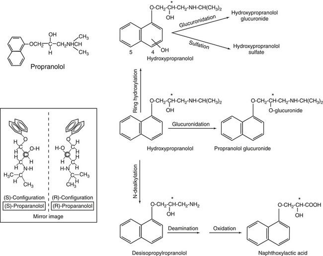
Figure 1-13 Propranolol offers an example of complex metabolism. Hepatic metabolism of propranolol follows multiple pathways, including both phase I (formation of hydroxyl propranolol) and phase Il (glucuronidation). Propranolol contains a chiral carbon (asterisk) resulting in enantiomers (inset). Each will potentially be metabolized by different pathways.
The sequela of phase I metabolism commonly is drug inactivation (e.g., phenobarbital). However, phase I metabolites often are equally, more (i.e., primidone or prodrugs, which must be activated such as enalapril), or less (e.g., diazepam, cyclosporine) active than the parent compound. More problematic, phase I metabolites often are reactive (e.g., oxygen radicals) and thus are more toxic (e.g., acetaminophen) than the parent compound (see Chapter 3).23,24 In such instances, phase II metabolism is critical to protecting the liver (or other metabolizing tissue) from metabolic products.
Phase II metabolism, also known as conjugation, occurs when a large water-soluble molecule is chemically added to either the parent drug or its phase I metabolite; this phase is often referred to as synthetic (see Figure 1-13). Generally, with the exception of glutathione transferase, phase II reactions require energy. As with phase I enzymes, families of enzymes catalyze each of the synthetic reactions. Glucuronidation is the most common phase II reaction; common substrates include OH and COOH functional groups (see Figure 1-13). The cat is deficient in some (but not all) glucuronide synthetic enzymes and as such does not eliminate phenols or carboxylic acids well (see Chapter 2). Glucuronide conjugates are eliminated in the urine and bile; degradation in the gastrointestinal tract and reabsorption of the substrate results in enterohepatic circulation. The glutathione transferase system targets electrophiles (compounds seeking electrons) and as such has several different roles in the body, including detoxification of radical metabolites. However, the enzyme can be rapidly depleted, which increases the risk of liver, red blood cell, or other tissue damage; n-acetylcysteine is a precursor for glutathione that can be used to replenish the system. Sulfonation targets hydroxyl groups and as such compensates somewhat for glucuronide deficiencies in cats. Acetylation is a less common synthetic reaction; sulfonamides are common substrates. The dog is a poor acetylator (see Chapter 2). With rare exceptions, phase II metabolites are inactive. The most common exception is with acetylation, which may result in formation of active metabolites (e.g., procainamide). Most hepatic drug metabolites are excreted in the urine, although some conjugated drugs undergo biliary excretion. Such drugs are potentially subject to enterohepatic circulation. Species (and no doubt breed) differences in both phase I and phase II metabolism are well recognized but insufficiently described (see Chapter 2).
Exogenous products are not the only substrates for drug-metabolizing enzymes. Many metabolic reactions are critical to formation or degradation of endogenous substances. Important noncytochrome metabolic enzymes include those that oxidize aldehydes or alcohols (esterases: e.g., acetylcholinesterases), monoamine oxidases (responsible for metabolism of endogenous catecholamines, dopamine, and related molecules) and dehydrogenases (alcohol and aldehyde) responsible for many endogenous reactions.
Factors that can affect hepatic drug metabolism include the amount and activity of drug-metabolizing enzymes and, if the drug is characterized by a high extraction ratio (>70%, a flow-limited drug), and hepatic blood flow. For flow-limited drugs, removal by drug-metabolizing enzymes is so rapid that the only limitation to the rate of elimination is blood flow. In contrast, extraction of capacity-limited drugs is slow. Protein binding directly decreases the clearance and thus rate of elimination of capacity-limited, but not flow-limited, drugs. Disease, drug interactions, and species differences can have a profound impact on drug metabolism and thus drug elimination (see Chapter 2).
Enantiomers and Drug Disposition
Whenever a carbon atom has four different structures bonded to it, two different molecules can be formed. Stereoisomers are chemical compounds with the same molecular formula that differ only by the orientation of functional groups in space around the central atom (e.g., carbon). Enantiomers are stereoisomers that differ due to orientation of four different groups around a single carbon (or phosphorous or nitrogen) atom and are nonsuperimposable mirror images of one another (Figure 1-14). The center atom around which the asymmetry occurs is referred to as the chiral molecule. The enantiomers are differentiated as to either D (dextrorotatory) or L (levorotatory). More commonly, they are defined by the direction in which they rotate light. As such, they are “optical isomers”: if one enantiomer rotates light to the left (S, or sinister [counterclockwise]), the other will rotate it to the right (R, rectus [clockwise]) the same number of degrees. The only physical difference between enantiomers is the direction in which they rotate light. However, although the physical characteristics of enantiomers are similar, the pharmacodynamics (including both potency and efficacy) and pharmacokinetics (all phases of disposition) may be profoundly different for each isomer. Most enantiomeric drugs are sold as racemic mixtures (generally 50:50), and administration of such drugs represents polypharmacy.25 Further complicating enantiomer disposition is the potential for each enantiomer to be converted to the other after administration. Species differences are likely to be profound. Unfortunately, analysis of enantiomers in tissue samples is difficult: they are so physically similar that their physical separation and thus quantitation from one another is difficult. Examples of drugs that exist as enantiomers include selected anthelmintics, verapamil, ketamine, inhalant anesthetics (isoflurane), selected cardiac drugs (e.g., beta blockers, including propranolol [see Figure 1-13], albuterol, and others), and a number of nonsteroidal antiinflammatories (e.g., the profens [ketoprofen, carprofen]). Occasionally, the name of a drug indicates it is a sole isomer (e.g., levofloxacin is the L isomer of ofloxacin.)
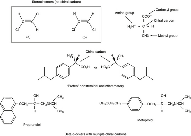
Figure 1-14 Enantiomers are stereoisomers that exist as mirror images that are not superimposable because of the presence of a chiral carbon (top). Rotation of the four groups attached to the chiral carbon results in either S or R isomers (depending on the rotation of light by each molecule). Although they are similar in MW and chemistry, the body often responds to and handles enantiomers differently. Most products are manufactured as racemic (1:1). Some compounds contain more than one chiral compound, complicating disposition. Further, interconversion among species contributes to the complexities that characterize the pharmacokinetics and thus predictability of disposition of these compounds. Examples of compounds that exist as stereoisomers include many nonsteroidal antiinflammatories (middle) or beta-blockers (bottom). Commercial products often contain mixtures of both enantiomers of a drug. However, some drugs are marketed as only the active enantiomer and are often named to indicate as such (e.g., “levo” as in levetiracetam or “dextro” as in dextromethorphan).
Excretion
Renal excretion is the most important route of drug elimination for both parent (especially water soluble) drugs and their metabolites (Figure 1-15).2,3,26,27 Host factors that determine renal excretion include renal blood flow (including glomerular filtration rate), active tubular secretion, and tubular (generally passive) reabsorption. The kidney is also capable of metabolizing some drugs (e.g., imipenem), although this capacity is only occasionally of clinical importance.
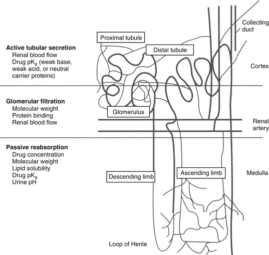
Figure 1-15 Renal excretion is the most common route of elimination of drugs and their metabolites. Three drug movements determine the rate of renal excretion. Active tubular secretion in the proximal tubule is a rapid process not limited by protein binding. Glomerular filtration is a passive process; protein-bound drugs cannot be filtered through the glomerulus. The rates of both active tubular secretion and glomerular filtration both depend on renal blood flow. Nonionized drugs that are sufficiently lipid soluble may be passively resorbed. Because urine drug concentration increases, passive resorption should also increase the concentration.
Glomerular filtration is a passive process. Drugs enter the glomerulus by bulk flow, being excluded if too large (> 60,000 MW) as occurs for highly protein-bound drug if the glomerulus is healthy. In contrast, active transport of drugs in the proximal tubules is very efficient, rapid, and insensitive to protein binding. However, it is susceptible to competition among drugs. Separate active transport (p-glycoprotein, OATPs, POTs) systems exist for acid, basic, and neutral drugs. Probenecid has been used clinically to compete with and thus inhibit the renal excretion of other weakly acidic drugs such as expensive beta-lactam antimicrobials (e.g., penicillin historically and imipenem more recently), thus prolonging therapeutic PDC. Reabsorption of drugs from renal tubules into peritubular capillaries slows renal excretion. The extent to which a drug is reabsorbed depends on its lipid solubility and its ionization. Weakly acidic drugs are more likely to be reabsorbed in acidic urine but are trapped and excreted in alkaline urine. Urinary pH can be therapeutically altered such that the renal excretion rate of a drug can be modified, particularly in cases of overdose or toxicity. Drugs excreted in the urine that do not undergo passive reabsorption will be progressively concentrated in the renal tubule. Tubular cells may be exposed to higher concentrations of drugs, which may increase the risk of nephrotoxicity. Drug concentration in the urine can be of therapeutic benefit in some situations, such as bacterial cystitis. Most antibacterials excreted in the urine achieve concentrations that exceed plasma at least tenfold (see Chapter 6); for such drugs, culture and susceptibility data and, in particular, minimum inhibitory concentrations based on PDC may underestimate efficacy if infection is limited to the urine.
In contrast to renal excretion, biliary excretion is very slow and much less clinically important. Drugs are eliminated in the bile by at least three active transport (p-glycoprotein) systems: one each for organic acids, organic bases, and organic neutral compounds. Characteristics that determine biliary excretion of drugs include chemical structure, polarity, and MW, with the latter being one of the major determinants (generally drugs >600 MW in size). Drugs excreted in the bile are in greater contact with the intestine and its flora compared with other drugs and are thus more likely to cause adverse reactions in the gastrointestinal tract. In addition, conjugated (phase II) drugs excreted by this route may undergo enterohepatic circulation (Figure 1-16) if intestinal bacteria unconjugate the drug or metabolite, allowing intestinal absorption to occur. Enterohepatic circulation prolongs drug elimination half-life and further exposes the gastrointestinal tract to drug.
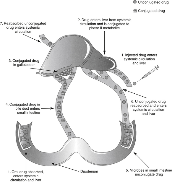
Figure 1-16 Enterohepatic circulation can prolong the elimination half-life of a drug. After oral or parenteral administration, the drug is conjugated in the liver and eliminated in the bile. The drug travels from the duodenum to the lower small intestine and colon. Bacterial degradation results in deconjugation of the drug, which can then be reabsorbed.
Elimination and Clearance
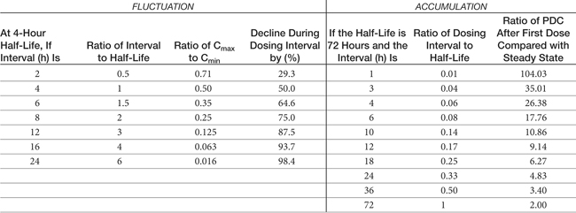
The combined effects of hepatic metabolism and renal and biliary excretion, as well as other routes of elimination not discussed (e.g., pulmonary, sweat), irreversibly remove or clear the drug from the body. Elimination refers to the disappearance of drug from plasma. Elimination half-life is among the more clinically relevant and the most often reported pharmacokinetic parameters. It is defined as the time necessary for plasma or blood concentrations to decline by 50%.28 Elimination half-life, however, is also dependent on Vd. Along with the therapeutic range, the elimination half-life should be the basis for an appropriate dosing interval. The amount of fluctuation in drug concentrations during a chosen dosing interval depends on the elimination half-life of the drug. Further, drug elimination half-life determines the time to steady state when either a drug (or new dose) is begun or discontinued. For example, at one drug elimination half-life, 50% of the dose has been eliminated; by five drug elimination half-lives, more than 97% of the drug has been eliminated (Figure 1-17, Table 1-1, and Box 1-2). Finally, the elimination half-life, along with the dosing interval, also determines the amount of drug that accumulates with each dose as steady-state equilibrium is reached (see the discussion of accumulation later in this chapter). This reflects first-order elimination, which might be considered a protective mechanism to ensure rapid elimination of potentially toxic substances.
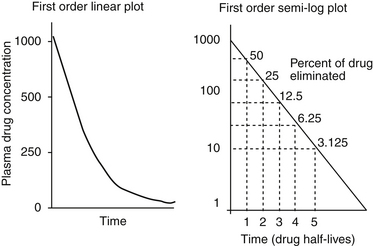
Figure 1-17 Drug elimination half-life can be derived from the plasma drug concentration versus time plot. Because most drugs are eliminated in a first order process (a constant fraction is eliminated per unit time), the amount of drug eliminated is concentration dependent. The relationship between concentration and time is linear when plotted on semilogarithmic paper but curvilinear when plotted on linear paper. The opposite is true for zero-order elimination (i.e., a constant amount is eliminated per unit time): The plot is linear on linear paper but curvilinear on semilogarithmic paper. For first-order elimination, if a line is drawn between two points (such as might be obtained from a peak and trough concentration), the line can be extrapolated to the y axis. The half-life is the time that elapses as plasma drug concentration decreases by half. Calculation of half-life is described in Box 1-3.
Table 1-1 Impact of Half Life and Dosing Interval on Fluctuation in or Accumulation of Plasma Drug Concentrations
Box 1-2 Zero- Versus First-Order Elimination
The importance of first-order (constant fraction) versus zero-order (constant amount; see Figure 1-17)29 elimination can be appreciated best in the context of the elimination rate constant. Assume an animal has ingested several aspirin to the point that the plasma drug concentration has surpassed the therapeutic range of 100 to 500 mg/mL and has achieved the toxic concentration of 2000 mg/mL. The half-life of aspirin in the dog is about 9 hours. First-order elimination results in a concentration of 1000 ng/mL by 9 hours and 500 ng/mL at 18 hours. Thus by 18 hours, the drug is back into the therapeutic range, and by 36 hours, it approximates the low therapeutic range. For zero-order elimination a constant amount is eliminated per unit time. For example, if 100 ng/mL of aspirin is eliminated every 9 hours, by the time 36 hours has elapsed, concentrations will have declined to only 1600 ng/mL.
Clearance is a parameter often used to assess the excretory capacity and thus physical well-being of an organ. Plasma clearance (CL) is the volume of plasma irreversibly cleared of the drug per unit time and represents the sum total of organ clearance (Figure 1-18) 2,3,30,31 As such, it is the most important of the pharmacokinetic parameters.32 Clearance differs from elimination because it is a volume per unit time, not a rate constant (amount per unit time). If the drug is cleared exclusively by one organ (e.g., renal clearance of aminoglycosides or hepatic clearance of caffeine), then plasma CL also represents clearance of the specific organ and can be used to evaluate the function of the organ. With first-order elimination, the volume of blood cleared per unit time by an organ is independent of PDC—that is, the same volume of blood will be irreversibly cleared of drug by an organ regardless of how much drug is in the blood. The exception occurs only if so much drug is present in the blood that the organ of clearance becomes saturated such that zero-order elimination emerges.
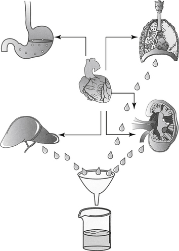
Figure 1-18 The clearance of drug from the body (plasma) is the sum total from each of the organs of clearance. Several organs not shown are also capable of drug clearance, most notably the skin.
Although clearance is the reason that PDC ultimately declines (thus is physiologically independent of any other factor), pharmacokinetically it is obtained or calculated from the volume to which the drug is distributed (Vd) and the rate at which the drug is eliminated from the volume (kel or half-life). Clearance can be calculated on the basis of compartmental modeling, or from AUC based on noncompartmental analysis (see the pharmacokinetics section). Despite its importance, practically, clearance is minimally useful in the design of dosing regimens other than through its impact on elimination half-life unless calculating a constant rate infusion. In contrast, half-life is the clinically useful estimate of how long a drug stays in the body. Yet, while half-life is the pharmacokinetic parameter measured directly from the PDC versus time curve, physiologically, it is a “hybrid” parameter in that it is affected by both distribution (Vd) and clearance (CL) (Box 1-3). The more rapidly a drug is cleared by an organ, the shorter the drug half-life. However, if a drug is distributed to a large tissue volume, PDC will be lower. Thus, although clearance (which is concentration independent) does not change, the volume cleared per unit time contains less drug and elimination decreases. If the Vd is much smaller, PDC is higher, more drug is in the volume of blood that is cleared. (see Figure 1-10). As such, the rate of elimination decreases. Thus drug elimination half-life changes directly and proportionately with Vd but inversely and proportionately with CL. The clinical significance of the relationship among Vd, CL, and half-life is exemplified in a patient who has renal disease and eventually becomes dehydrated as a result of uncompensated chronic renal disease. Initially, as renal function declines, a smaller volume of blood goes through the kidney, which thus clears less blood. Drug elimination half-life decreases. However, as the patient becomes dehydrated, blood and ECF volume contracts, and the Vd decreases. As a result, PDC increases such that more drug is in each volume of blood as it is cleared. Thus in the patient with both fluid volume contraction (half-life decreases) and compromised renal function (half-life increases), drug half-life may not change from normal even though renal function may be impaired. With volume replacement (i.e., fluid therapy), Vd will increase, causing half-life to increase because less drug is now in the smaller volume that is being cleared.
Half-life of any drug movement can be determined in several ways. Half-life can be directly determined from a drug concentration versus time graph by measuring the distance on the X axis (time) that occurs as PDC (Y axis) decreases by 50% (see Figures 1-20 and 1-23). More often, half-lives for each component of a drug concentration versus time curve are determined from each slope, or rate constant, ki: At one half-life (t2−t1 = t1/2), the drug concentration declines by 50%. Thus at t2- t1, C1/C2 = 2. However, because drug concentrations (Y axis) are natural logs, C1/C2 becomes the natural log (ln) of 2 = 0.693. Thus the rate constant or slope of any line ki = 0.693/ t1/2. Conversely, if the rate constant is known, t1/2 = 0.693/ki. In the same manner, half-life also might be calculated from peak and trough concentrations collected from a patient (see Chapter 5). The slope, or ki, is simply the rise/run, or (C1 − C2)/(t2 − t1) where C is the concentration of sample 1 or 2 and t is the time that samples 1 and 2 were collected (see Figure 1-20). Because concentration is logarithmic, the actual equation becomes

For example, if gentamicin samples collected at 2 hours and 12 hours after an intravenous dose were 10.5 and 2.0 mg/mL, respectively, the kel for gentamicin in this animal would be 0.17 h−1 and the elimination half-life would be calculated at 4.2 hours.
Fixed Dosing Regimens
Dose
A fixed dosing regimen comprises a route, a dose, and an interval (or frequency)(see Box 1-3). The dose necessary to achieve a specified target PDC (e.g., Cmax) following a single dose depends on the volume of tissue that will dilute the dose administered, estimated by Vd:2,3

The dose of drug must be increased or decreased proportionately with changes in Vd to achieve the same target PDC (or C0 or Cmax)(see Figures 1-10 and 1-19). Often, the dose is not intended to reach Cmax but rather Cmin (e.g., phenobarbital) or midway between the two extremes of the therapeutic range. The concentration within a therapeutic range that is selected as the target depends on the drug efficacy and safety. The Vd of a drug is the sole determinant of PDC for single doses of an intravenously administered drug. With multiple dosing the relationship between elimination half-life and dosing interval also may influence PDC (see later discussion). For extravascular drugs, bioavailability also must be considered, with the dose inversely but proportionately influenced by bioavailability:
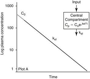
Figure 1-19 Plasma drug concentration (PDC) versus time curves after intravenous administration. This drug could be described by a one-compartment open model because it plots as a single straight line (one slope) on semilogarithmic paper. There is no initial distribution phase, and the volume of distribution is based on PDC extrapolated (dotted line) from the first concentration measured back to time zero (C0). The equation for this single component curve would be Cp = Coe–kt where Cp is the plasma drug concentration at any time and t and k are the elimination rate constants (slope) of the curve. Such behavior is unusual for a drug because it implies instantaneous distribution from plasma to tissues or failure to leave circulation. The latter might happen if a drug is very tightly bound to plasma proteins and total, rather than unbound drug, is measured.

By definition, with intravenous administration, F= 1, or 100% bioavailability.
Interval
The relationship between elimination half-life and dosing interval determines the amount of fluctuation in PDC during a dosing interval. This relationship has several clinical implications (see Table 1-1 and Figures 1-20 and 1-21). The shorter the elimination half-life compared with the dosing interval, the greater the fluctuation. The dosing interval for a drug is based on the time (Tmax) it takes for PDC to decline from the peak concentration achieved after dosing (Cmax) to the lowest concentration that occurs during the dosing interval (Cmin) (see Figures 1-20 through 1-22). Thus the interval depends on the amount of fluctuation in PDC allowed during the dosing interval and the half-life of the drug, or its inverse (0.693/t1/2), the elimination rate constant (kel). If Cmin for a drug is close to half of Cmax, then approximately one drug half-life (i.e., Tmax = t1/2) can elapse before the next dose should be administered. A more appropriate interval can be calculated with kel if Cmin does not approximate half of Cmax:
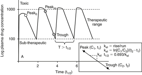
Figure 1-20 Plasma drug concentration versus time curves after multiple extravascular dosing for a drug that is administered at a dosing interval substantially longer than the elimination half-life. Such a drug is less likely to accumulate because most of the drug will be eliminated during a dosing interval. For such drugs equilibrium between tissue and plasma concentrations is never reached and steady state is not really relevant. The risk of toxicity and therapeutic failure is a potential concern with each dose, unless the dosing interval is shortened such that fluctuation during the dosing interval is minimized. For monitoring, a peak and trough concentration may be necessary. The inset demonstrates how the half-life of a drug might be calculated from drug concentrations measured at two time points after administration of a dose.
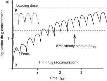
Figure 1-21 Plasma drug concentration versus time curves following multiple extravascular dosing for a drug that is administered at a dosing interval substantially shorter than the elimination half-life (see also Figure 1-16). The amount that the drug accumulates as steady state is reached determines the drug concentration at steady state and is based on the magnitude of difference between dosing interval (T) and drug half-life (t1/2). Such a drug will accumulate because most of the drug from the previous dose is still in the body by the next dose. Although equilibrium may not be truly reached, steadystate (characterized by the same Cmax and Cmin at each dosing interval) occurs after three to five drug half-lives have elapsed after administration at the same dose, interval and route. For some drugs, if a rapid therapeutic response is desired, a loading dose can be given. Note, however, that steady state has not been reached and plasma drug concentration may increase or decrease as steady-state is reached if the maintenance dose is not correct. When monitoring is done for such drugs, generally a single sample collected at any time during the dosing interval is sufficient to reflect the whole dosing interval.
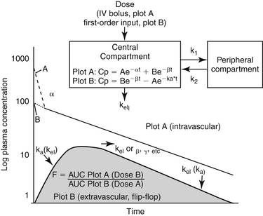
Figure 1-22 After intravenous administration, a drug distributed to peripheral tissues generally is characterized by at least two components or phases when plotted on semilogarithmic paper. According to compartmental modeling, the plasma drug concentration (PDC) declines in the first phase (component) due to both distribution into tissues and back and elimination (excretion) from the body. Once a distribution equilibrium (pseudo-equilibrium) has been reached, PDC decline is caused only by elimination (second phase or component of the curve). The two phases can be separated by stripping and residual analysis, or linear regression. The first (stripped and subsequently fitted) component of the curve (coarse dotted line) is understand to represent distribution, and the slope (α) is the distribution rate constant. The slope of the second phase of the curve is the elimination rate constant (kel). The equation for the curve represented by plot B (two components) can be used to determine the concentration of drug in plasma (or the tissue being sampled) at any time (t) by the equation: Cp= Ae–αt+Be–βt. The volume of distribution (Vd) for this drug is ideally based on PDC after distribution, usually determined by extrapolating (fine dotted line) the terminal or elimination phase of the PDC versus time curve (B on plot A) yielding Vd area or Vd extrapolation. The Vd based on the extrapolated concentration for the first component of the line (A on Plot A) might be used to calculate the central volume (Vc) to which the drug is immediately distributed. The second PDC versus time curve (Plot B) reflects extravascular (e.g., oral) administration of the same dose of drug. The upswing of the PDC versus time curve reflects the simultaneous movements of absorption, distribution and elimination from the body, all occurring during first-order input (a constant fraction moves per unit time). As each movement reaches pseudoequilibrium (amount moving either way is the same), remaining movements that have not yet reached equilibrium emerge. Of the movements, elimination from the body will not reach equilibrium (open model) and as such, emerges as the terminal movement or component. The absorption rate constant (ka) can be derived from the upswing of the curve but only after the elimination component of the curve has been mathematically stripped. Generally, the distribution phase of nonintravenous doses is masked by the absorptive phase. The equation of extravascular PDC versus time curves follows the general equation: Cp = Be–βt – Ae–ka t where A is the extrapolated drug concentration from the absorptive phase of the curve; it is subtracted from the overall equation because it represents the area that is “missing” from the curve as the drug is being absorbed. The elimination rate constant of a drug should be the same, regardless of the route of elimination. However, in some cases the rate of absorption is so slow that it limits the rate of elimination. As such, the absorption rate constant determines the slope of the terminal curve (i.e., ka and kel are “flip-flopped,” as is demonstrated in the figure). A flip-flop model should be suspected if the elimination rate constant after extravascular administration is significantly less than that after IV administration. As such, a flip-flop model can be ascertained only if the drug is give intravenously. If IV administration is not done to affirm the terminal slope as kel, it should be reported as the disappearance rate constant, kd. IV administration is also necessary to determine Vd,CL and absolute bioavailabililty (F) of a drug. (see Box 1-6.)

The longer the elimination half-life of a drug, or the wider the difference between Cmax and Cmin, the longer the possible interval (or Tmax) between doses. Understanding the relationship between dosing interval and elimination half-life can help determine which aspect of the dosing regimen (i.e., close or interval) should be changed when trying to improve drug response by either increasing PDCs or minimizing fluctuation during the interval. Through altered kinetics in the patient, two scenarios are offered.
The first scenario is dosing with a drug at an interval that is close to or longer than the drug elimination half-life. With this scenario, prolonging a dosing interval (e.g., for convenience) may allow drug concentrations to fluctuate excessively during the dosing interval and may result in either adverse events as Cmax is approached with each dose or therapeutic failure as Cmin is approached just before each subsequent dose. Note that wide fluctuation between Cmax and Cmin may not necessarily be undesirable. For example, if the drug is effective despite nondetectable drug concentrations, the interval can be longer than the half-life might dictate. Examples include concentration-dependent antimicrobials (e.g., aminoglycosides), drugs that accumulate in tissues (e.g., omeprazole), drugs such as diazepam whose metabolites are active (some with drug half-lives longer than that of the parent compound), and drugs whose effects are irreversible (e.g., receptors or enzymes are destroyed (e.g., aspirin and thromboxane synthetase).
On the other hand, if the drug is characterized by a narrow therapeutic window, fluctuation should be minimized and a shorter interval may be indicated. To add one half-life to the dosing interval, the dose must be doubled; however, to add subsequent half-lives, the dose must be doubled each time. Thus to add three half-lives to a dosing interval, the dose must be increased eightfold (23) (e.g., time dependent drugs or anticonvulsants). Some drug half-lives are short on the order of minutes (e.g., epinephrine). Constant rate infusion may be indicated if an intravenous preparation is available such that therapeutic concentrations can be maintained for a clinically relevant period while avoiding the negative consequences of undesirable fluctuations in PDC that might occur with convenient dosing intervals (see later discussion). Manufacturers have provided an alternative approach to maintenance of PDCs for drugs with a short half-life by formulating the drug in a preparation characterized by slowed absorption (e.g., extended release preparations) or (less commonly) distribution. However, even if absorption is prolonged, once the drug enters circulation, it’s elimination half-life is the same. Absorption of a drug might be slowed by several methods. Examples of parenteral slow-release preparations include drug-esters (drug is released by esterases at the site of administration) or liposomal or other products that release drug as the product is degraded. Oral methods include extended- or delayed-release products consisting of capsules that degrade at different rates. Note, however, that absorption may be so slow that therapeutic concentrations are never reached. Many preparations used in animals have been formulated for humans, and the release kinetics may vary substantially in animals. A less common mechanism of constant drug input is slow release from circulating plasma proteins for a drug that is highly protein bound (e.g., cefovecin).
A second scenario is a drug administered at an interval that is much shorter than the half-life. For such drugs, little drug may be eliminated during the dosing interval, and shortening the interval will be beneficial only if an additional dose is added (rather than dividing the same daily dose into more dosing periods). For example, assume the half-life of phenobarbital approximates an average of 72 hours. Dividing the dose into 8- rather than 12-hour intervals offers no advantage because 3 days must lapse for 50% of the drug to be eliminated. Indeed, a 24-hour dosing interval may be sufficient for most patients, unless induction of drug-metabolizing enzymes causes the half-life to markedly decrease (see Chapter 2). For drugs with very long half-lives, depending on the Cmax and Cmin of the drug, dosing intervals generally can be correspondingly long. However, a dosing interval that is too long might result in too much fluctuation in PDC during a dosing interval, which may be problematic for drugs characterized by a narrow therapeutic window. It also might lead to noncompliance if the owner forgets to medicate. In both situations the recommended dosing interval is often shorter than the drug elimination half-life. In such instances the drug will accumulate, and the concept of steady state and the potential need for a loading dose must be addressed (see below).
Accumulation
If a drug is administered at an interval that is approximately three half-lives, most (87.5%) of the drug will be eliminated between each dose. However, if the interval is shorter, some drug from the previous dose will still be present in the plasma when the next dose is given. Indeed, if the drug is administered at an interval that equals the half-life, 50% of the previous dose is still in the body when the next dose is given. Thus if each subsequent dose of drug is administered at an interval (T) that is equal to or shorter than the drug half-life, most of the previous dose is still in the body, and the drug accumulates with multiple doses (see Figures 1-17 and 1-21).2,3 Eventually, a steady state is reached such that the amount of drug administered with each dose equals the amount eliminated during the dosing interval. As with drug elimination, approximately three to five drug half-lives must elapse following a fixed dosing regimen before steady state is reached. Note that steady state is a relevant issue only for drugs that accumulate—that is, the drug is administered at a dosing interval that is shorter than the drug elimination half-life. The amount of accumulation can be described by the accumulation ratio (R), which describes the magnitude of the drug concentration following the first dose compared with that at steady state (Css); the ratio can be applied to Cmin, Cmax, or Caverage (R = Css/C1st).
Just as the amount of fluctuation between Cmin and Cmax depends on the relationship between half-life and interval (i.e., for a drug dosed at an interval shorter than the half-life), the accumulation ratio also depends on the relationship between dose and interval, being logarithmically proportional to the difference between the two: R = 1/1– e –kel∗ T where R = the accumulation ratio, T = the dosing interval and kel = the elimination rate constant (see Figure 1-21 and Tables 1-1 and 1-2). The dosing regimen of drugs that accumulate is generally designed so that drug concentrations will be in the therapeutic range at steady state. If the elimination half-life is equal to the dosing interval, although PDC will fluctuate twofold between doses, the drug will also accumulate twofold (i.e., Cmax at first dose:Cmax at steady state = 2) as steady-state is reached.The greater the half-life compared with the dosing interval, the more the drug will accumulate (see Table 1-2). Using the example of phenobarbital, as drug is begun, the elimination half-life may approximate 72 hours (kel=0.693/72 h). When the seventh dose is given 72 hours later, 50% of the first dose still remains. Based on a 72-hour half-life and 12-hour dosing interval, an accumulation ratio of 9 is expected. Thus if peak PDC following the first dose of 3.5 mg/kg was 2 μg/mL, concentrations of 18 μg/mL would be expected at steady state 9 to 14 days later. Because drug concentrations fluctuate very little for drugs that accumulate, missed doses should present minimal risk of therapeutic failure. The missed dose can simply be given with the next dose. However, to change PDCs substantially, multiple doses (i.e., a “miniloading” dose) must be given. When monitoring, a single sample collected at any time during the dosing interval should accurately reflect PDC throughout the dosing interval because concentrations change minimally during the interval.
Table 1-2 Rate of Drug Accumulation Based on the Length of the Dosing Interval (T) Compared with Elimination Half-Life (t½)
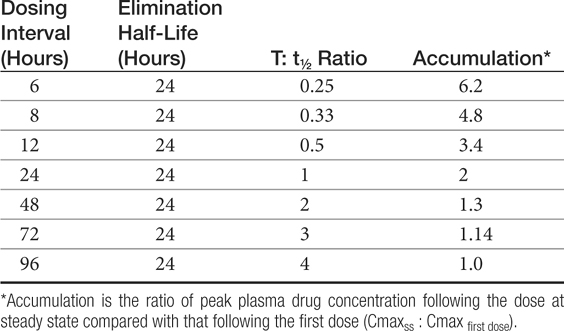
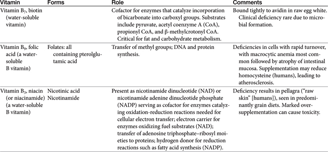
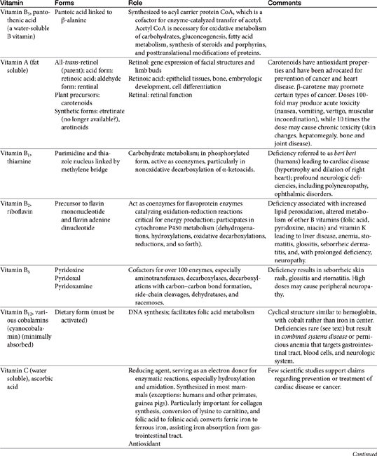
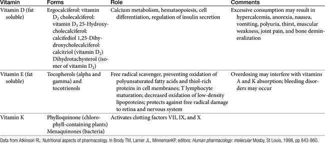
With a 21-day half-life in dogs, bromide offers an extreme example of accumulation when dosed once daily. At steady state, bromide concentrations will be 35 times what they were after the first dose. Likewise, during a 24-hour dosing interval, fluctuations in PDC will be so small that they should not be detectable. Levetiracetam, on the other hand, offers an example at the other end of the spectrum: With a 2-hour half-life, 87% of the drug may be eliminated during an 8-hour dosing interval. Missed doses may put the patient at risk for therapeutic failure, and monitoring might best include both a peak and trough sample. If only one sample can be collected, a trough sample might be sufficient because the drug is so safe. However, if side or adverse effects are of concern with the drug (e.g., clorazepate), both a peak and trough sample might be collected for drugs with a short half-life compared with the dosing interval.
Clinically, drugs that accumulate present another problem not encountered with drugs administered at an interval that precludes accumulation. Maximum therapeutic efficacy is not realized until steady-state concentrations are reached, which may be an unacceptable time for some patients (e.g., epileptics receiving potassium bromide [KBr]) (see Figure 1-21). In such situations a loading dose can be administered with the intent of achieving therapeutic concentrations with a single dose or, in the case of bromide, several days of dosing. Note, however, that a loading dose does not achieve steady state. Steady state is achieved only after the drug is administered at the same dose for three to five drug half-lives. As such, although a properly calculated loading dose will result in PDCs immediately achieving the therapeutic range, the maintenance dose must be designed to maintain these concentrations. A loading dose should be considered only when therapeutic response depends on steady-state concentrations and the time to this point is unacceptable (i.e., three to five drug half-lives). The benefits of loading (i.e., a rapid response) should be weighed against the risk of adverse events that will be increased if the body does not have time to accommodate to high drug concentrations. Further, pet owners are not likely to understand the concept of loading and may either forget to modify or intentionally continue a loading dose, the latter because they wrongly assume that a higher dose can be tolerated longer.
A loading dose always is accompanied by a maintenance dose; the maintenance would be the same regardless of whether a loading dose is administered concurrently because it also is designed to achieve therapeutic concentrations at steady state. The maintenance dose should “match” the loading dose—that is, it should be designed to maintain what the loading dose achieved. The maintenance dose, not the loading dose, determines PDC at steady state: By the time steady state is reached (three to five half-lives), the loading dose will have been eliminated. However, at one half-life, while 50% of the loading dose will have been eliminated, 50% of steady-state concentrations will have been achieved. If the maintenance dose fails to maintain what the loading dose achieved, PDC will either decline (maintenance dose too small) or increase (dose too great) as steady state is achieved. Either miscalculation can lead to therapeutic failure. The greatest decrease (or increase) will occur during the first elimination half-life after loading is completed; as such, inappropriate patient response may occur at one half-life.
The loading dose is calculated according to the (apparent) Vd at steady state (Vdss) of the drug and the targeted PDC at steady state, Css (mg/mL). Thus for drugs with 100% bioavailability (e.g., intravenously administered drugs):

The dose can be adjusted for less than 100% bioavailability by:
Using bromide as an example, the minimum effective concentration (Cmin) is 1 mg/mL (1 gm/L). With a Vd of 0.3 L/kg, and near 100% oral bioavailability, a loading dose intended to achieve the minimum therapeutic range would be Cmin∗ Vd/F or (0.3 l/kg) ∗ (1 gm/L)/1 or 300 mg/kg. Because potassium bromide is only 69% bromide (potassium MW = 35; bromide MW = 79), the dose of potassium bromide necessary to achieve 1 mg/mL is 300 mg/kg/0.69 = 433 (rounded up to 450 mg/kg). Note that he loading dose of bromide that targets 1 mg/ml at steady-state is much higher than the daily maintenance dose (approximately 30 mg/kg per day) that would achieve 1 mg/mL at steady state (approximately 2.5 months of dosing). The difference between the loading dose of a drug and its maintenance dose reflects the difference between the elimination half-life and the dosing interval. Simplistically, the loading dose should reflect all the doses that would be given as the drug reaches steady state, less the amount eliminated during that same time period. The longer the elimination half-life, the larger the loading dose compared to the maintenance dose.
Constant-rate infusion (CRI) offers an example of a drug that is administered at an interval that is much shorter than the half-life (Box 1-4). For CRI the rate is infinitely small. The rate of infusion (ROI or ko) should result in an input that equals the output. Output will be described by (total body) clearance (CL; ml/kg/hr) of the drug: ROI (mg/kg/h) = CL × Css (see pharmacokinetics section). Because clearance, in turn, reflects the volume of blood from which drug is eliminated per unit time (CL = Vd ∗ kel), then ROI = Css ∗ Vd ∗ kel. Further, because kel can be calculated from half-life, then ROI = Css ∗ Vd ∗ (0.693/t1/2). When calculating CRI, care must be taken to ensure that units are converted such that they match. Note that increasing the ROI will increase the total concentration achieved at steady state but will not increase or decrease the time to steady state. As with any other dosing scheme, steady state will not be achieved with a CRI until three to five elimination half-lives have elapsed, which may be unacceptably long. As such, a loading dose may be indicated when administering a CRI if patient response time is too long. Note, however, that a sufficient clinical response may occur well before maximum drug concentrations are achieved at steady-state. Likewise, the time for drug concentrations to decline after a CRI is discontinued will be based on the same elimination rate constant: Three to five drug half-lives must elapse before the drug is eliminated from the body, although clinical response may resolve well before all the drug is entirely eliminated.
Box 1-4 Calculation of a Constant-Rate Infusion for Fentanyl
In normal dogs, the volume of distribution (Vd) of fentanyl ranges from 4 to 10 L/kg and its t1/2 ranged from 2.5 to 6 h. Using an average Vd or 7 L/kg and 3h as the t1/2, then kel = 0.693/3 = 0..35 hr-1 and clearance (CL) becomes (0.173 hour-1 ∗ 7 L/kg) = 2.45 L/kg/h (2450 mL/kg/h to match units). To target Cmin or 1 ng/mL (or 1 μg/L) of fentanyl at steady state (9-15 hours), the rate of infusion (ROI or Ro) = ([1 ng/mL] ∗ 2450 mL/kg/h) = 2450 ng/kg/h (2.45 μg/kg/h) or 0.04 μg/kg/min. If the half-life is 3 hours, steady-state concentrations should be reached in approximately 9 to 15 hours. Although analgesic relief may not require steady-state concentrations, safety of the constant-rate infusion cannot be fully assessed until steady state is reached. If the time to steady state is too long, 1 ng/mL (Cmin) can be immediately reached by an administration of a loading dose (DL): DL = Css ∗ Vd = (5 L/kg ∗ 1 μg/L) or 5 μg/kg, which can be administered as an intravenous bolus.
Extrapolation of dosing regimens among species for drugs that accumulate is more difficult than for drugs that do not. For drugs that do not accumulate, dose is largely based on Vd and, if not administered intravenously, bioavailability (which can be difficult to extrapolate among species). However, for drugs that accumulate, if the drug is given in multiple doses, both Vd and elimination half-life must be taken into account for intravenous drugs, along with bioavailability for nonintravenous drugs.
Pharmacokinetics
The quantitative description of drug movements in the body is referred to as pharmacokinetics. Pharmacokinetic modeling is used to predict the behavior of a drug in the body. Generally, the drug of interest is given at the desired route of administration as a single dose, and drug concentrations are collected over time, preferably for at least three elimination half-lives to ensure that all phases of drug movement are identified. For bioavailability studies, the drug should be given intravenously (100%) as well as by the route of interest, ideally using a randomized crossover paired design. For drugs intended for multiple dosing, particularly chronically, pharmacokinetic analysis also should take place across the intended duration of therapy to detect changes in drug disposition over time. Several methods of pharmacokinetic modeling are used to study drug movements; the most common described in the veterinary literature are either compartmental or noncompartmental analysis; population pharmacokinetics represents an emerging variation.2,3,9,33 Boxes 1-3 to 1-6 provide some useful pharmacokinetic equations.
Compartmental Analysis
Compartments
Plotting of PDC versus time data on semilogarithmic paper linearizes the data for most drugs because drug movements follow first-order kinetics—that is, a constant fraction rather than a constant amount (zero order) of drug moves (is absorbed, distributed, or excreted) per unit time. For first-order behavior, the amount of drug per unit time varies with the concentration of drug, whereas with zero-order elimination (as might occur when metabolism enzymes are saturated), the amount eliminated per unit time is concentration independent. Theoretically, after administration, each movement to which the drug is subjected occurs at a different rate: absorption and distribution are generally faster than elimination. Each movement results in a change in the slope of the curve, with each slope thus reflecting a different drug movement or combination of movements. Intravenous drug administration yields a PDC versus time curve that begins with the highest PDC (see Figures 1-19 and 1-22).
After intravenous administration (no absorption), data described by a single component (i.e., only one slope or rate; see Figure 1-19) is interpreted to indicate that only one compartment or drug movement occurs, which is elimination from the body (excretion Such a behavior might describe a drug whose distribution is either instantaneous (or occurs before the first sample is collected) or is limited to plasma (i.e., highly protein bound drug). The model is described as a one-compartment open (meaning drug can move into or out of compartments) model. More commonly, two drug movements characterize the time course of the drug in the body (see Figure 1-22, plot A). For such drugs, PDCs initially decline because of the combined effects of two drug movements: distribution to (and from) tissues and excretion (elimination) from the body. Because distribution is generally more rapid, elimination emerges after distribution equilibrium (pseudo-equilibrium) is reached (i.e., the amount of drug moving into tissue equals the amount of drug leaving the tissue). Beyond that point, less drug is leaving the plasma because changes in PDC reflect only one drug movement, excretion (elimination from the body). The elimination is slower (the slope is flatter). Data for such drugs is characterized as a two-compartment open model.2,3,9 More than two compartments may emerge as drug behavior is modeled. Drugs also can be bound to peripheral tissues. For such drugs the time to distribution to well perfused tissues may reach equilibrium more rapidly than to the deeper peripheral tissues, and the PDC versus time curves may be composed of three or more components: the terminal component presumably reflecting elimination from the body, the next component potentially reflecting distribution to a “deep” compartment, and the initial component reflecting distribution to “peripheral” compartments.
If a drug is given via an extravascular route (e.g., orally, intramuscularly, subcutaneously), the initial change in PDC is characterized by an increase (see Figure 1-22, plot B; non-intravenous). Once absorption is complete, drug concentrations decline as elimination becomes the primary drug movement (see Figure 1-22, plot B; nonintravenous). Because absorption generally is slower than distribution, the latter is often “masked” by the absorptive phase and can not be mathematically determined. Thus, extravascular administration may be characterized only by two drug movements, absorption and elimination (one compartment open model with first order input). It is important to note that the assignment of each component or compartment of the PDC versus curve to a specific drug movement is theoretical. While conceptually, this approach to modeling makes sense, other models also can describe the data without compartmentalization (e.g., physiologic).
Mathematical Description
In order to pharmacokinetically describe or model drug behavior, thus allowing prediction of drug concentrations at any time, the time course of drug movements is reduced to one equation that best describes, or “fits” the data. If the data are best described by multiple compartments, each component should be described uniquely in the equation. Thus to distinguish the rate constant and Y intercept of one movement from those of another, each slope must be separated or “stripped” from the combined curve. Each component of PDC can be manually separated from the previous component. To do so, the terminal-most component is first extrapolated to the Y axis, and the “predicted” Y values on that line are subtracted from the “actual” data on the PDC versus time curve. The residuals (predicted) are plotted at the same time points, and a new line is drawn to represent the next (proximal) component of the curve. The process is repeated for each component until the initial component has been identified. The process of residual analysis is tedious; as such, computer-generated programs generally strip the data and identify the components. Each component that results from stripping is then subjected to linear regression to determine the equation that best describes each component of the time versus PDC relationship. Thus, one of the disadvantages of compartmental analysis is that predicted data, rather than actual data, may be the basis for determining pharmacokinetic parameters. This does not represent a problem unless the predicted data are not a good “fit”; poorly fitting data will contribute to the variability of the data. Scientific papers that describe the pharmacokinetics of a drug on the basis of compartmental analysis should provide an assessment (e.g., sum of residuals) of how well the actual data fit the “best” predictive line resulting from linear regression, thus providing an indication of the relevance of the predicted parameters to actual parameters. The advantage of compartmental analysis is that each component may reflect a different drug movement (absorption, distribution, or elimination), thus elucidating drug behavior. However, no matter how good the fit, the labeling of a component of the curve with a drug movement is theoretical and may not actually reflect what occurs in the body. Further, the labeling of each of the components of the curve with a drug movement, although routinely done, is theoretical: modeling does not assure the first component is distribution, the next elimination, etc.
Once separated, each component of the PDC versus time curve is described by a Y intercept (Co if one compartment [see Figure 1-19], A and B if two compartments [see Figure 1-22, plot A], or A, B, and C for three compartments, and so forth) and a rate constant (kel for one compartment or α, β, or γ, and so forth, for multiple compartments). The Y intercept for each component is determined by extrapolation of the line of each component (beginning with the terminal-most) back to the Y axis. For a one-compartment model, the extrapolated Y intercept is generally referred to as Co to indicate plasma drug concentrations at time 0. For multiple components each succeeding component is not extrapolated until that portion of the line has been stripped from the distal component. The units of PDC as extrapolated to Y are weight/volume (i.e., μg/mL, mg/mL, mg/L, and so on). The rate constant (or slope) describes the percentage change per unit time for each component. The rate constant of the terminal-most component is generally referred to as kel but also referred to as β if a two-component curve, γ with three components, and so on. Alternatively, the slopes or rate constant may simply be referred to as λ (lambda; i.e., λ1, λ2, λz, etc with λz being the terminal component) as a reminder that assignment of movements is theoretical. The units of rate constants are the inverse of time (time–1, e.g., min–1). The rate constant of the initial component of the curve following intravenous administration is generally referred to as α and the distribution rate constant.
Once the Y intercept and slope of each curve is identified, the PDC versus time curve, regardless of the number of components, can be described by the following basic equation: (Cp) = Coe-kt, where Cp is the plasma drug concentration at any time, t; Co is the instantaneous plasma drug concentration (before distribution or elimination have occurred, extrapolated from the appropriate component of the curve), and k is the respective elimination rate constant (slope of the line). This equation is simply the semilogarithmic (because movements are first order) version of the equation for a line, Y= mx + B where Y is the concentration (Cp) at any time X (t), m is the (logarithmic) slope of the line (e-k), and B is the Y intercept (Co) (Box 1-5).
Box 1-5 Parameters for Compartmental Analysis
Plasma drug concentrations (Cp), at any time (t) after administration. For open model, after intravenous administration:
One compartment: Cp = Coe–kt (Figure 1-19)
Two compartment: Cp = Ae–αt + Be–βt (Figure 1-22)
Three compartment: Cp = Ae–αt + Be–βt+ Ce–γt.
For first order input (extravascular): Cp = Be–kel∗t – Ae–ka∗t
Area under the curve (AUC): One compartment: AUC = A/α; (or Co/ kel). Two compartment: AUC = A/α + B/β: three compartment: AUC = A/α + B/β+ C/γ. Units for AUC are reflected in its determinants: plasma drug concentrations represented by the respective Y intercepts Co, A B, C, and so on, reported in weight/volume (e.g., mg/L or μg/mL), and the respective rate constants (α, β, γ, and so on for intravenous administration and ka for the absorptive phase of extravascular administration; reported in inverse time or time–1[e.g., min–1]).
Area under the moment curve (AUMC): A/α2 for one compartment; A/α2 + B/β2 for a two-compartment model, and so on).
(Apparent) Volume of Distributions (Vd): Vc (volume of the central compartment), VdB, Vd area, and Vdss; > VdB > Vd area > Vdss > Vc.): Units of volume/mass (e.g., L/kg) reflect the dose (generally mg/kg) and extrapolated drug concentration (C0 or B). The Vd of a drug can be determined only after intravenous administration because bioavailability = 100 %; if F is known, Vd can be calculated substituting D ∗ F for D in each of the equations.
Vd B = Dose/B (Figure 1-22, Figure 1-23)
Dose (D) (units generally mass/mass, e.g., mg/kg):
Intravenous administration: D = Co ∗ Vd
Extravascular administration: D = Co ∗ Vd/F
Clearance (CL): The CL of a drug represents the fraction of the Vd of a drug that is cleared per unit time (kel). Thus if the Vd and kel (or half-life) of a drug are known, the CL of the drug can also be determined: CL = Vd • kel Because CL is calculated from Vd, it can be determined only after intravenous administration of a drug (unless F is known).
A similar approach to modeling is taken for extravascular data, which must be described by at least two components. The slope of the upswing of the PDC versus time curve (once stripped from the distribution or elimination components of the curve) describes the absorption rate constant, designated ka; the Y intercept must be determined after all other components of the curve are stripped (see Figure 1-22). For extravascular administration, the model would be referred to as a one-compartment open model with first-order input, indicating that the rate of absorption, like the rate of elimination, is first order. If the decline in PDC after the absorptive phase revealed two slopes, the model would be two compartments, with the first compartment or component possibly representing distribution that was slower than absorption. For some drugs (including extended- or delayed-release preparations), the rate of absorption is slower than the rate of elimination. For such drugs, absorption is reflected in the terminal-most, rather than initial, component of the PDC versus time curve and the elimination rate constant for such drugs is determined from the upswing of the PDC versus time curve. Such drugs are generally said to follow a “flip-flop” model and can be identified only after intravenous administration because it is only through this route that the effects of absorption are removed from the terminal component of the curve (see Figure 1-22). Drugs exhibiting a flip-flop behavior are characterized by a terminal rate constant following intravenous administration that is statistically shorter than the terminal rate constant measured after non-IV administration.
Area under the Curve (AUC)
Once the equation of the PDC versus time curve of a drug has been established, a number of parameters can be determined to further describe or explore drug behavior (see Box 1-5). Among the more important parameters generated from pharmacokinetic analysis is the AUC, a parameter that indicates duration and extent of exposure of a drug after administration of a specific dose. Following compartmental analysis, AUC is calculated by dividing the Y intercept of each slope by the rate constant of the slope; for multiple compartments the terms are additive. Thus, for a one-compartment model, AUC = A/α; (or Co/ kel); for a two-compartment model, AUC = A/α + B/β, and so on (see Figure 1-22). The units for AUC are reflected in its determinants: PDC (Co, A, B, and so on) of mg/mL (or weight/volume) and a rate constant (inverse time or time–1: min–1). An example would be an AUC of 546 mg ∗ min/mL.
AUC is used to calculate several other parameters important to the description of drug behavior. Area under the moment curve (AUMC: A/α2 for one-compartment model, A/α2 + B/β2 for a two-compartment model, and so on) is a parameter with little physiologic relevance, but it is used to calculate other parameters. Among the more important parameters based on AUC is bioavailability, the percentage of a drug that reaches systemic circulation. Absolute bioavailability is determined by measuring the AUC after nonintravenous administration (see shaded area of plot B in Figure 1-22) and comparing it with the AUC measured after intravenous administration (100% absorption), with differences in doses adjusted for as needed. Rather than presented as a percentage, bioavailability is often presented as a ratio (F) and, as such, is unit-less. If the AUC for both curves is equal, bioavailability is 100% (F = 1) (Box 1-6).
Box 1-6 Bioavailability Calculation
Bioavailability (F, unitless) is the percentage of a drug that reaches systemic circulation. Absolute bioavailability is determined by measuring the area under the curve (AUC) after nonintravenous administration and comparing it with the AUC measured after intravenous administration (100% absorption), with differences in doses adjusted for as needed (see Figure 1-22): F = [AUC X] ∗ [Dose IV] / [AUC IV ] ∗ [ Dose X], where X is the nonintravenous route of administration (Figure 1-22). Relative bioavailability can be compared between different nonintravenous routes in the same manner.
Rate Constants and Half-lives
Generally, because each component of the curve is associated with a specific drug movement, the half-life is also associated with that movement (e.g., absorption, distribution, or elimination [disappearance] half-lives), each referring to the time necessary for 50% of the respective drug movement to be complete (or reach equilibrium). Of the drug movements, elimination from the body is generally the slowest. As such, the elimination half-life is represented by the slope of the terminal, or final component, of the PDC versus time curve. However, this assignment can only be confirmed with IV administration since the terminal component of non-IV administration may reflect absorption (i.e., a flip-flop model). If an intravenous dose is not studied, the terminal component may be referred to as a disappearance rate constant or half-life. The distribution half-life is generally calculated from the initial component of the curve (generally referred to as α) following intravenous administration; the distribution component of the curve is often masked with oral administration. Absorption half-life is derived from the ka unless a flip-flop model has been identified. Note that the faster the absorption half-life, the higher Cmax and shorter Tmax, the time to the maximum concentration. Because half-life is calculated from the inverse of kel (t1/2 = 0.693/kel) (see Box 1-4), half-life from a sample population cannot be normally distributed. As such, reports providing descriptive statistics should be reported as harmonic mean (derived from averaging the inverse of each half-life, [1/HL + 1/HL…] and reinversing the mean) and pseudo standard deviation is generally reported.
Volume of Distribution
The dose of a drug is based on the target concentration and the volume of tissue to which the drug appears to be distributed. The actual volume of tissue distribution cannot be calculated. However, the Vd is a theoretical volume to which the drug is distributed (or the volume of tissue that dilutes a drug), assuming that the drug concentration throughout the body is the same as that measured in plasma. Because this is unlikely, and because it is mathematically derived, the Vd of a drug is referred to as apparent. The Vd of a drug is calculated by administering a known dose intravenously and dividing it by the maximum PDC that occurs after the drug is distributed but before any elimination occurs: Vd = Dose/PDC (Co) (Figure 1-23). Because dose is generally in milligrams per kilogram and C0 (or B) is generally milligrams per milliliter (the same as grams per liter), Vd is generally reported as liters per kilogram. The Vd of a drug can be determined only after intravenous administration in order to ensure that all drug reaches systemic circulation (i.e., bioavailability = 100 %). Occasionally, if a drug is not given intravenously, scientific articles or drug package inserts might report Vd/F, indicating the Vd corrected for bioavailability that is less than 100% (F<1). However, the clinical relevance of this parameter largely depends on knowledge of bioavailability.
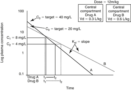
Figure 1-23 Changes in volume of distribution (Vd) affect plasma drug concentration and the slope of the elimination (kel) curve that determines elimination half-life. The former is impacted because movement of drug into tissues removes it from plasma and thus organs of elimination. Plot A represents PDC versus time following administration of a dose of drug in an animal with a Vd that is half of that represented in plot B (compartment size increased in the latter). Note that the slope of the plasma elimination curves for animal B is flatter. As such, elimination half-life also will be longer. Drug half-life can be determined by measuring the time (t2 - t1) necessary for PDC to decrease drop 50% (C1 to C2).
The Vd of a drug is primarily used to calculate the dose of the drug (see Box 1-5). Three different Vds are reported in the literature. Because the PDC cannot be measured immediately (before distribution and elimination influence the curve), the PDC used to determine Vd must be derived after the terminal component is extrapolated to the Y intercept (see Figure 1-22). If the plasma elimination curve yields only one component (e.g., distribution from plasma does not occur or is instantaneous), PDC is extrapolated to time 0 or C0, yielding the volume of the central compartment (Vc). This volume can be used to determine the initial concentration of a drug (e.g., to assess potential toxicity) or to estimate plasma volume. However, for many drugs distribution is not instantaneous and the PDC versus time curve is multicomponent. To remove the effects of elimination that occur during distribution, the terminal component of the PDC is then extrapolated to the Y axis. Generally referred to as B if the model is two-compartment, this PDC theoretically reflects peak PDC after distribution has reached equilibrium (pseudo-equilibrium) but prior to elimination. The Vd after distribution has reached pseudo-equilibrium then becomes Vd = Dose/B, often referred to as Vd area, Vd extrapolated, or Vdβ. For multicomponent curves, Vc can still be determined using the extrapolated initial component of the curve using A (or C0): Vc = Dose/C0 or Dose/A (see Figure 1-22).2,3,12,30,34,35 Because Vd area is influenced by clearance (it is based on extrapolation of the terminal elimination curve), it tends to overestimate the true volume. It is useful to predict the amount of drug that remains to be excreted at any time point during elimination.17 The third Vd is that which occurs at steady state, when equilibrium has been reached (Vdss). True equilibrium can be reached only if clearance does not occur, or if input equals output, as might occur with CRI.17 As such, Vdss is independent of clearance and more accurately reflects the true volume diluting the drug. (see Box 1-5).
The Vd, although a calculated parameter, is used to calculate clearance, which is the physiologic action that is responsible for the elimination of drug (see Box 1-5). As with Vd, CL/F may be reported in studies for which an intravenous drug was not administered. However, this is not a clinically relevant parameter unless bioavailability has been demonstrated to be 100% for the animals in the study in question or unless bioavailability is known. Although generally calculated, clearance can be measured. However, collection requires repeated sample of the tissue into which drug is cleared. Plasma clearance of a drug that is cleared exclusively through the urine can be determined by sequentially sampling urine rather than plasma or, as with creatinine clearance, collecting a volume of urine into which the drug has cleared and plasma samples containing the drug at the beginning and end of the sampling time. Determining clearance of a drug excreted in the bile would require biliary catheterization.
Noncompartmental Analysis
All models are, by definition, incorrect. Thus, a disadvantage of compartmental analysis is that data (particularly poor fitting data) is forced to fit the “best” equation that mathematically describes the data (Box 1-7). The more variable the data, the more inaccurate compartmental analysis is because the greater the deviation of actual data from predicted data. Noncompartmental analysis often is used in lieu of compartmental analysis, particularly if rate constants are not necessary to describe the behavior of a drug in the body. Further, no attempt is made to relate noncompartmental pharmacokinetic parameters with physiologic processes, thus reducing confusion or bias that might occur with interpretation. For noncompartmental analysis the primary parameter determined is AUC. This parameter can be determined in a variety of ways, but the most common (for noncompartmental analysis) is the trapezoidal method (Figure 1-24).33,34 For this method a series of sequential trapezoids are drawn, each defined by a line drawn between two subsequent data points in the PDC versus time curve. The remainder of the trapezoid is determined by dropping the lines from each data point on the line to the X axis. The area for each trapezoid is determined, and areas are summed to generate AUC. The last trapezoid can end at either the last actual time point measured or be extrapolated “to infinity” based on the slope of the terminal component of the data. As with compartmental analysis, the elimination rate constant (terminal component of the curve) and thus half-life is based on the best-fit analysis. However, all other remaining parameters are based on AUC. As such, mean residence time, MRT, is a comparable, more physiologically descriptive and thus preferred parameter to elimination half-life. Based on AUC, MRT describes the average time a molecule is in the body (or the time necessary for 63.2% of a drug to be eliminated). The difference between MRT after intravenous versus extravascular administration is the mean absorption time, MAT, providing a noncompartmental method for assessment of the absorptive phase of the drug.
Box 1-7 Parameters for Noncompartmental Analysis
(From Martinez MN: Special series: use of pharmacokinetics in veterinary medicine, Article II: volume, clearance, and half-life, J Am Vet Med Assoc 213:1122-1127, 1998.)
Mean residence time: MRT = AUC/AUMC (area under the curve/area under the moment curve)
Clearance (intravenous only): CL = dose/AUC
Extravascular: CL and volume of distribution (Vd) must be corrected for bioavailability by multiplying by D ∗ F. For extravascular administration, mean absorption time (MAT) describes the absorptive phase of the drug movement; however, it can be determined only if the drug is also studied intravenously (MAT = MRTEV- MRTIV where EV = extravascular).
Vd at steady state (intravenous only): Vdss = Vdss: (D × AUMC)/ AUC2 (∗ Extravascular: Vdss: (D ∗ F x AUMC)/AUC2)
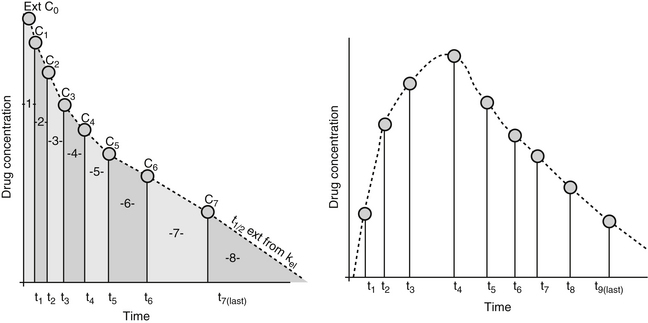
Figure 1-24 For noncompartmental analysis the area under the curve is determined by adding the area calculated for the trapezoids formed by two adjacent data points. If AUC is determined to infinity, the terminal component is based on the slope of the terminal time points as determined by linear regression. The advantage of noncompartmental analysis is that actual data points are used rather than predicted data. As with compartmental analysis, the more data points, the more accurately the data is likely to represent the actual time course.
Alternative Pharmacokinetics
Pharmacokinetic studies generally are implemented in a sample population of the target species by administration of a dose via the intended route and subsequent intermittent collection of tissues (generally blood, representing the central compartment, but occasionally specific tissues representing peripheral/compartments), that are subjected to quantitative analysis of the drug and or its metabolites. The number of animals and samples from each animal must be sufficient for accurate description of the time course of drug concentrations in the sampled tissue. The more the data points, the better the data represents the population. The approval process for animal drugs does not necessarily require pharmacokinetic modeling of drugs; if required, generally the studies are performed in normal animals. Pharmacokinetics for human drugs are performed in humans, with studies involving dogs most often focusing on toxicity. Data often are available only through Freedom of Information Act publications. Population pharmacokinetics study the sources of variability in drug concentrations among patients, and as such the science takes advantage of multiple studies that differ in study design or subjects. Further, population pharmacokinetics can take advantage of data collected in patients, which generally is restricted because of ethical considerations that might limit the study to small sample numbers.35 With limitations, a pharmacokinetic profile of a drug might also be generated for the individual patient using this approach (Chapter 5).
Other Considerations
Dosing Based on Allometric Scaling and Body Surface Area
Allometry refers to the phenomenon of changes in shape that result from changes in size. Allometric scaling attempts to predict a change in physiologic response based on a change in another physiologic parameter. Over 34 anatomic, physiologic (including heart rate, blood volume, and glomerular filtration), and biochemical parameters correlate with body weight across species; not surprisingly, body weight has been extensively examined as a method of allometrically scaling for species differences in physiologic processes. Using the allometric equation Y = a Wb, many physiologic parameters (Y) do appear to be predicted by weight (W) adjusted with an allometric exponent (b) of 0.67 to 1. The usefulness of adjusting doses on the basis of body weight scaled according to body surface area (BSA = 10 – W2/3) was initially realized in children receiving drugs characterized by a narrow therapeutic index.37,38
As with children, the simplest method of dosing based on body weight, tends to underdose small animals and overdose larger animals, and the use of BSA should improve accuracy of dosing. Because animals differ so much in body shape as well as size, the equation can be further normalized by the addition of the shape constant K: BSA = K • 10 – W2/3. The formula is most commonly applied to cancer chemotherapeutic drugs, with the supposition that large-breed dogs would benefit most (thus preventing the relative overdosing they received compared with smaller dogs). However, because the incidence of adverse reactions to cancer chemotherapeutic drugs increased in smaller dogs compared with larger dogs using this approach, the method needs to be reassessed. Several observations made by Price and associates36 help support the need to re-examine the application of the method to all animals. First, studies have suggested that the mass exponent used to correct weight (2⁄3 or 0.67) is incorrect. Other studies have shown that the exponent may vary as a function of age. This and other factors suggest that a range of mass exponents should be applied to animals within the same species. Second, although studies have shown that the allometric scaling of doses does help normalize doses among species, normalization using the same shape constant (K) within species has not been documented. Although a single K may be appropriate for the domestic cat, marked differences should be expected for the dog. Indeed, previous literature reveals that a number of shape constants have been used in dogs, ranging from 9.9 to 12.3 (Appendix 2), with the smaller value being applied to smaller or more compact dogs. It may be necessary to apply different constants to growing animals.
Using allometric scaling based on body weight or BSA, even adjusted for body shape, as a method of predicting dose (which incorporates both pharmacodynamics and pharmacokinetics) is likely to be difficult; many aspects of drug disposition seemingly are not related to BSA or body weight. These include protein binding; effects of pH on drug movement; actions of p-glycoprotein (i.e., active tubular secretion in renal tubular cells); differences in the composition of body compartments; and, most dramatically, differences in the rate, extent, and type of drug-metabolizing enzymes among the species. One study evaluated the allometric relationship between body weight and drug elimination half-life. Because half-life is equally affected by Vd and clearance, it serves as a good parameter to assess the overall relationship. Not surprisingly, those drugs whose half-lives are most likely to be predicted by allometric scaling tended to be minimally protein bound, characterized by a Vd indicative of distribution to ECF and excreted renally in the unchanged but also undergoing flow-limited hepatic extraction;38 many antimicrobials meet these criteria. Half-life tended to be less correlated allometrically with body weight for drugs that were highly protein bound, distributed to specialized body compartments, or metabolized by the liver in a capacity-limited fashion.37,38 Additional studies are needed to identify the most appropriate factors to be used to allometrically scale dosing regimens. To date, use of weight adjusted to BSA appears to be the most reasonable method for smaller animals.
Routes of Administration
Choice of the route and technique of administration is generally based on several factors, including the physicochemical properties of the drug, formulation to be used, therapeutic indication, pathophysiology of the disease, and the target species. The manufacturer’s recommendations should always be followed carefully unless it is explicitly known that a proposed deviation will not adversely alter the activity or kinetic fate of the principal ingredients. Note that regardless of the dosage form used, it is imperative to have an appreciation of the makeup of the pharmaceutical formulation, the factors that may alter the efficacy of the product, and the best way to derive optimal therapeutic benefit from the agent without jeopardizing its bioavailability or pharmacologic action.
Oral Administration
The United States Pharmacopeia provides an excellent source of currently accepted dosing forms.38 Common oral dosage forms include tablets, capsules, boluses, powders, granules, syrups, solutions, suspensions, and pastes. Oral bioavailability of oral dosing forms may profoundly differ. Other specialized delivery systems are also available, including enteric-coated tablets and sustained-action or controlled-release preparations. However, if designed for human use, their behavior in animals may be substantially different, particularly if orally administered. The advantages of oral dosing are that it is usually convenient and safe, sterility is not a requirement, and the danger of acute drug reaction is not as great as with intravenous administration. The disadvantages include a slower onset of action and unpredictability and inconsistency of absorption, including the sequela of exposing the drug to the unstable gastrointestinal tract. Additionally, dosing may be difficult in fractious animals, poor technique or dysphagia may lead to intratracheal delivery and subsequent bronchopneumonia, and inactivation may occur within the gastrointestinal tract. Some drugs may cause esophageal damage, particularly in cats.
Parenteral Administration
The most common parenteral dosage form is a stable aqueous solution. Less frequently, the active components may be dissolved in an inert vegetable oil, which delays absorption. Other kinds of prolonged-release preparations include subcutaneous implants of solid dosage forms and relatively insoluble salts and esters as suspensions in various vehicles. It is important to appreciate the basic differences between these and standard pharmaceutical preparations. First, accidental intravenous administration can lead to serious and even fatal effects related to microembolism. Second, persistent drug residues in racing or other show animals may have ethical and legal ramifications. The stability of solutions intended for parenteral administration often is delicate, depending on pH, temperature, and the presence of stabilizers, solubilizers, and preservatives. Indiscriminate mixing of such products for the sake of convenience (e.g., single versus multiple injections) should be avoided unless proof exists that the formulations are physically and chemically compatible. Several novel approaches for the parenteral delivery of drugs are being developed, including microspheres, microcapsules, liposomes, microsponges, resealed carrier erythrocytes, and projectile biodegradable missiles. Additionally, monoclonal antibodies have been used to carry highly selective, bound drugs to specific target tissues or even cells. Implantable controlled-release drug delivery systems include pellets (composed of various polymeric forms) and silicone capsules. Several implantable devices also have been introduced that permit constant systemic delivery of a drug within the body; these include osmotically or propellant-driven pumps and mini pumps. The advent of nanotechnology is likely to markedly improve drug delivery to targeted tissues. Liposomes are the earliest example of drug delivery systems based on nanotechnology; more current products include polymer-drug conjugates.
The most frequently used parenteral routes are intravenous (IV), intramuscular (IM), and subcutaneous (SC). Common but less frequently used routes include epidural, intradermal, intratracheal, and intraperitoneal (IP). Occasional routes of injection include intraarterial, intramedullary, intrathecal, intrathoracic, subarachnoid, intracardiac, subconjunctival, and intratesticular. Intralesional injection is a way of attaining high concentrations of a drug at the target site. In all cases solutions for injection must be sterile, techniques must be aseptic, and the dose must be accurate; a painful reaction is a possibility. For the IV route, aqueous solutions are preferable, which lead immediately to predictably high blood levels with a rapid onset of action. Irritating and nonisotonic solutions can be injected intravenously if done slowly and carefully. Usually, but not always, drugs given intravenously can be given intramuscularly or subcutaneously, but injection may be painful (e.g., arginine vehicles, or other basic or acidic solutions). Further, IM absorption of some IV drugs (e.g., diazepam) is not predictable. The IM route can be used for aqueous or oleaginous suspensions, solutions, and other depot preparations. Absorption occurs either hematogenously or by way of lymphatics and usually is fairly rapid except in the case of long-acting preparations. The addition of esters can variably prolong absorption depending on the rate of hydrolysis. Acetate salts are more slowly hydrolyzed than succinate salts (e.g., glucocorticoids); benzathine salts are more slowly hydrolyzed than procaine salts (e.g., penicillin). Moderately irritating preparations can be injected intramuscularly, but tissue reaction and necrosis may become evident with time. The duration of drug action is longer than for IV injection but most often is slightly shorter than for SC administration; however, this is not always predictable. A disadvantage of the IM route is the possibility of improper deposition in nerves, blood vessels, fat, or between muscle bundles in connective tissue sheaths. The advantages of the SC route are similar to those of the IM route, although irritant preparations and oily vehicles should be avoided due to possible undesirable reactions. The rate of absorption from SC injection sites may be unpredictable and depends on several factors. The most important of these is blood flow, and the presence of vasoconstrictors or vasodilators can substantially alter rates of absorption. Usually, the rate of absorption is slightly slower than from IM sites.
Miscellaneous Parenteral Routes
The other parenteral routes of administration are generally used for the following purposes: epidural and subarachnoid for spinal analgesia and myelography; intradermal testing for hypersensitivity and for vaccination; intratracheal treatment of respiratory tract infections; intraarterial with simultaneous venous constriction, with the latter causing high concentrations of drug in the dependent area for a short time (occasionally necessary in cancer chemotherapy and special radiographic or other imaging techniques); intramedullary (blood transfusion or fluid therapy directly into the bone marrow) when other routes are awkward, as in neonates; intrathecal (cisterna magna) for treatment of meningoencephalitis and myelography; intrathoracic (intrapleural or intrapulmonary and); and intracardiac for emergencies, especially cardiac arrest.
Inhalation (pulmonary route)
Gases, volatile agents, and fine particles usually are rapidly absorbed from the airways and alveoli into the pulmonary circulation. Delivery into the respiratory passages is done by standard anesthetic machines in the case of inhalation anesthetics or by vaporization or nebulization for the local delivery of expectorants, bronchodilators, and antiinfective agents. Drugs in the gaseous state readily reach the alveolar surfaces, whereas only particles less than 2 μm (produced by nebulization) are inspired into the terminal ducts and alveoli. Particles less than 5 μm may reach the respiratory bronchioles, and those 5 to 10 μm in size may reach the upper respiratory tract and larger airways. Because the depth of airway penetration is influenced by depth of respiration (directly) and respiratory rate (inversely) as well as the tortuosity of the airways, aerosolization generally should not be the sole route of administration of drugs in animals. Aqueous solutions of antibacterial drugs intended for injection may be delivered intratracheally. Absorption of drugs may occur after topical administration in the respiratory tract.
Topical administration (local application)
Drugs can be applied topically to the skin and its adnexa or to a variety of mucous membranes. The routes that may be used include sublingual, intranasal, intravaginal, intrauterine, intracystic, rectal, preputial, ocular, and aural. Many dosage forms have been developed to deliver active principles to the site of application to produce local effects. However, in many instances absorption into the systemic circulation also occurs. A wide variety of preparations are available for dermal application, including ointments, creams, pastes, dusting powders, lotions, sprays, liniments, and poultices. Systemic effects may occur as a result of the animal licking at the applied medication or due to percutaneous drug absorption, which often occurs, especially when the skin is damaged or inflamed (e.g., burns, ulcers, wounds, dermatitis). Absorption through the skin can also be enhanced by occlusive dressings, inunction, or the use of dimethyl sulfoxide (DMSO) as a carrier. Several drugs are deliberately applied to the skin with the anticipation of systemic effects after transdermal absorption—for example, transdermal gels, ectoparasiticides available as “pour-on” formulations, nitroglycerin ointment, and scopolamine in a transdermal patch device as well as iontophoresis devices. Of these the pluronic-lecithin transdermal gels, which are generated through compounding pharmacies, appear to be minimally effective for all but a few drugs and their use is not recommended unless specifically supported by scientific studies.
Transmucosal administration
Transmucosal or buccal drug administration represents a variation of oral administration (see previous discussion of topical administration). Drugs are given by mouth with the intent of absorption occurring through the mucosa of the mouth. A major advantage of this route of administration is avoidance of first-pass metabolism, which occurs with drugs that are swallowed. Convenience may be an additional reason. In contrast to the skin, mucosal tissues do not contain a stratum corneum, and therefore drugs are not presented with a significant barrier to movement into vascular tissues. Several methods of transmucosal delivery have been studied in dogs, including transmucosal gels (often with carboxymethylcellulose as the carrier), sprays, and patches. Among the difficulties associated with transmucosal administration in animals is maintaining contact time between drug and surface.
1. Lees P., Cunningham F.M., Elliott J. Principles of pharmacodynamics and their applications in veterinary pharmacology. J Vet Pharmacol Ther. 2004;27:397-414.
2. Ritschel W.A., Kearns G.L. Handbook of basic pharmacokinetics including clinical applications, ed 5. Philadelphia: Hamilton Drug Intelligence Publications; 1999.
3. Rollins D.E. Pharmacokinetics and drug excretion in bile. In: Benet L.Z., Massoud N., Rowland M., editors. Clinical pharmacokinetics: concepts and applications. Philadelphia: Lea & Febiger, 1989.
4. Toutain P.L., Lees P. Integration and modeling of pharmacokinetic and pharmacodynamic data to optimize dosage regimens in veterinary medicine. J Vet Pharmacol Ther. 2004;27:467-477.
5. Beal S.L., Benet L.Z., Benowitz N.L., et al. Pharmacokinetic basis for drug treatment. New York: Raven Press; 1984.
6. Baggott J.D. Principles of drug disposition in domestic animals. In: Baggott J.D., editor. The basis of veterinary clinical pharmacology. Philadelphia: Saunders; 1977:73-112.
7. Kim R.B. Drugs as p-glycoprotein substrates, inhibitors and inducers. Drug Metab Rev. 2002;34:47-54.
8. Mealey K.L. Therapeutic implications of the MDR-1 gene. J Vet Pharmacol Ther. 2004;27:257-264.
9. Notari R.E. Biopharmaceutics and clinical pharmacokinetics: an introduction, ed 4. New York: Marcel Dekker; 1987.
10. Toutain P.L., Bousquet-Mélou A. Bioavailability and its assessment. J Vet Pharmacol Ther. 2004;27:455-466.
11. Schentag J.J. Correlation of pharmacokinetic parameters to efficacy of antibiotics: relationships between serum concentrations, MIC values, and bacterial eradication in patients with gram-negative pneumonia. Scand J Infect Dis. 1991;74(Suppl):218-234.
12. Martinez M.N. Special series: use of pharmacokinetics in veterinary medicine, Article IV: clinical application of pharmacokinetics. J Am Vet Med Assoc. 1998;213:1418-1420.
13. Kunta J.R., Sinco P.J. Intestinal drug transporters: in vivo function and clinical importance. Curr Drug Metab. 2004;5:109-124.
14. Craig W.A., Ebert S.C. Protein binding and its significance in antibacterial therapy. Infect Dis Clin North Am. 1989;3:407-414.
15. Belpaire F.M., DeRick A., Dello C., et al. Alpha 1-acid glycoprotein and serum binding of drugs in healthy and diseased dogs. J Vet Pharmacol Ther. 1987;10:43-48.
16. Toutain P.L., Bousquet-Mélou A. Free drug fraction vs. free drug concentration: a matter of frequent confusion. J Vet Pharmacol Ther. 2002;25:460-463.
17. Toutain P.L., Bousquet-Mélou A. Volumes of distribution. J Vet Pharmacol Ther. 2004;27:441-453.
18. Bergan T. Pharmacokinetics of tissue penetration of antibiotics. Rev Infect Dis. 1981;3:45-66.
19. LeFrock J.L., Prince R.A., Richards M.L. Penetration of antimicrobials into the cerebrospinal fluid and brain. In: Ristuccia A.M., Cuhna B.A., editors. Antimicrobial therapy. New York: Raven Press; 1984:397-413.
20. Schenkman J.P., Kupfer D. Hepatic cytochrome P-450 monooxygenase system. New York: Pergamon Press; 1982. pp 99-156
21. Parkinson A. Biotransformation of xenobiotics. In: Klaassen C.D., editor. Casarett and Doull’s toxicology: the basic science of poisons. ed 5. New York: McGraw-Hill; 1996:113-186.
22. Bogaards J.J.P., Bertrandoe M., Jacsonoe P. Determining the best animal model for human cytochrome P450 activities: a comparison of mouse, rat, rabbit, dog, micropig, monkey and man. Xenobiotica. 2000;30:1131-1152.
23. Guengerich F.P. Cytochrome P450 and chemical toxicology. Chem Res Toxicol. 2008;21:70-83.
24. Mitchell J.R., Smith C.V., Lauferburg B.H., et al. Reactive metabolites and the pathophysiology of acute lethal cell injury. In: Mitchell J.R., Homing M.G., editors. Drug metabolism and drug toxicity. New York: Raven Press; 1984:301-318.
25. Landoni M.F., Soraci A.L., Delatour P., et al. Enantioselective behavior of drugs used in domestic animals: a review. J Vet Pharmacol Ther. 1997;20:1-16.
26. Somogyi A. New insight into the renal secretion of drugs. Trends Pharmacol Sci. 1987;8:354-357.
27. Bekersky I. Renal excretion. J Clin Pharmacol. 1989;27:447-449.
28. Toutain P.L., Bousquet-Mélou A. Plasma terminal half-life. J Vet Pharmacol Ther. 2004;27:427-439.
29. Dayton P.G., Cucinell S.A., Weiss N., et al. Dose-dependence of drug plasma level decline in dogs. J Pharmacol Exp Ther. 1967;158:305-316.
30. Martinez M.N. Special series: use of pharmacokinetics in veterinary medicine, Article II: volume, clearance, and half-life. J Am Vet Med Assoc. 1998;213:1122-1127.
31. Martinez M.N. Special series: use of pharmacokinetics in veterinary medicine, Article V: clinically important errors in data interpretation. J Am Vet Med Assoc. 1998;213:1564-1569.
32. Toutain P.L., Bousquet-Mélou A. Plasma clearance. J Vet Pharmacol Ther. 2004;27:415-425.
33. Nestorov I. Whole-body physiologically based pharmacokinetic models. Expert Opin Drug Metab Toxicol. 2007;3(2):235-249.
34. Gabrielsson J., Weiner D. Pharmacokinetic and Pharmacodynamic Data Analysis: Concepts and Applications. Stockholm: Swedish Pharmaceutical Press; 2000. Sweden
35. Guidance for Industry: Population Pharmacokinetics. Accessed May 05, 2010. http://www.fda.gov/downloads/Drugs/GuidanceComplianceRegulatoryInformation/Guidances/ucm072137.pdf
36. Price G.S., Frazier D.L. Use of body surface area (BSA)-based dosages to calculate chemotherapeutic drug dose in dogs, I. Potential problems with current BSA formulae. J Vet Intern Med. 1998;12:267-271.
37. Riviere J.E., Martin-Jimenez T., Sudlof S., et al. Interspecies allometric analysis of the comparative pharmacokinetics of 44 drugs across veterinary and laboratory animal species. J Vet Pharmacol Therap. 1997;20:453-463.
38. United States Pharmacopeia, National Formulary, General Chapter 1151.