Computed Tomography
At the completion of this chapter, the student should be able to do the following:
1 List and describe the various generations of computed tomography (CT) imaging systems.
2 Relate the CT imaging system components to their functions.
3 Discuss image reconstruction via interpolation, back projection, and iteration.
4 Describe CT image characteristics of image matrix, Hounsfield unit, and sensitivity profile.
5 Describe technique selection in CT.
6 Explain the helical imaging relationships among pitch, index, dose profile, and patient dose.
7 Discuss image quality as it relates to spatial resolution, contrast resolution, noise, linearity, and uniformity.
THE COMPUTED tomography (CT) imaging system is revolutionary. No ordinary image receptor, such as screen film or an image-intensifier tube, is involved. A collimated x-ray beam is directed on the patient, and the attenuated image-forming x-radiation is measured by a detector whose response is transmitted to a computer.
After the signal from the detector is analyzed, the computer reconstructs the image and displays the image on a monitor. Computer reconstruction of the cross-sectional anatomy is accomplished with mathematical equations (algorithms) adapted for computer processing.
Helical CT, which has emerged as a new and improved diagnostic tool, provides improved imaging of anatomy compromised by respiratory motion. Helical CT is particularly good for the chest, abdomen, and pelvis, and it has the capability to perform conventional transverse imaging for regions of the body where motion is not a problem, such as the head, spine, and extremities.
This chapter introduces the physical principles of multislice helical CT. Special imaging system design features and image characteristics are reviewed.
The components necessary to construct a computed tomography (CT) imaging system were available to medical physicists 20 years before Godfrey Hounsfield first demonstrated the technique in 1970. Hounsfield was a physicist and engineer with EMI, Ltd., the British company most famous for recording the Beatles, and both he and his company justifiably have received high acclaim.
Alan Cormack, a Tufts University medical physicist, shared the 1979 Nobel Prize in physics with Hounsfield. Cormack had earlier developed the mathematics used to reconstruct CT images.
The CT imaging system is an invaluable radiologic diagnostic tool. Its development and introduction into radiologic practice have assumed an importance comparable with the Snook interrupterless transformer, the Coolidge hot-cathode x-ray tube, the Potter-Bucky diaphragm, and the image-intensifier tube. No other development in x-ray imaging over the past 50 years has been as significant.
Principles of Operation
When the abdomen is imaged with conventional radiographic techniques, the image is created directly on the screen-film image receptor and is low in contrast, principally because of Compton scatter radiation. The intensity of scatter radiation is high because of the large area x-ray beam. The image is also degraded because of superimposition all of the anatomical structures in the abdomen.
For better visualization of an abdominal structure, such as the kidneys, conventional tomography can be used (Figure 28-1). In nephrotomography, the renal outline is distinct because the overlying and underlying tissues are blurred. In addition, the contrast of the in-focus structures has been enhanced. Yet the image remains rather dull and blurred.
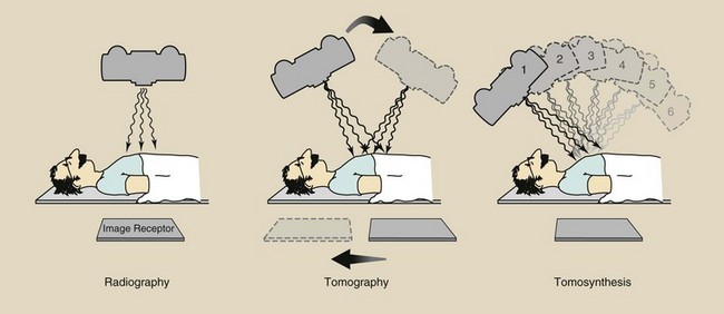
FIGURE 28-1 Equipment arrangement for obtaining a radiograph, a conventional tomography, and a digital radiographic tomosynthesis image set.
The latest advance in digital radiography is digital radiographic tomosynthesis. This imaging technique uses an area x-ray beam to produce multiple digital images. The images form a three-dimensional data set from which any anatomical plane can be reconstructed. The result is even better image contrast.
Conventional tomography is called axial tomography because the plane of the image is parallel to the long axis of the body; this results in sagittal and coronal images. A CT image is a transaxial or transverse image that is perpendicular to the long axis of the body (Figure 28-2). Coronal and sagittal images can be reconstructed from the transverse image set.
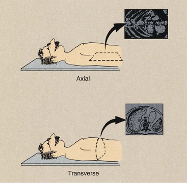
FIGURE 28-2 Conventional tomography results in an image that is parallel to the long axis of the body. Computed tomography (CT) produces a transverse image.
The precise method by which a CT imaging system produces a transverse image is extremely complicated, and understanding it requires strong knowledge of physics, engineering, and computer science. The basic principles, however, can be observed if one considers the simplest of CT imaging systems, which consists of a finely collimated x-ray beam and a single detector. The x-ray source and the detector move synchronously.
When the source-detector assembly makes one sweep, or translation, across the patient, the internal structures of the body attenuate the x-ray beam according to their mass density and effective atomic number, as was discussed in Chapter 9. The intensity of radiation detected varies according to this attenuation pattern, and an intensity profile, or projection, is formed (Figure 28-3).
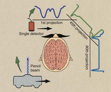
FIGURE 28-3 In its simplest form, a computed tomography (CT) imaging system consists of a finely collimated x-ray beam and a single detector, both of which move synchronously in a translate and rotate fashion. Each sweep of the source detector assembly results in a projection, which represents the attenuation pattern of the patient profile.
At the end of this translation, the source detector assembly returns to its starting position, and the entire assembly rotates and begins a second translation. During the second translation, the detector signal again will be proportional to the x-ray beam attenuation of anatomical structures, and a second projection will be described.
If this process is repeated many times, a large number of projections are generated. These projections are not displayed visually but are stored in digital form in the computer. Computer processing of these projections involves effective superimposition of each projection to reconstruct an image of the anatomical structures within that slice.
Superimposition of these projections does not occur as one might imagine. The detector signal during each translation has a dynamic range of 12 bits (4096 gray levels). The value for each increment is related to the x-ray attenuation coefficient of the total path through the tissue. Through the use of simultaneous equations, a matrix of values is obtained that represents the transverse cross-sectional anatomy.
Generations of Computed Tomography
The previous description of a finely collimated x-ray beam and single detector assembly that translates across the patient and rotates between successive translations is characteristic of first-generation CT imaging systems. The original EMI imaging system required 180 translations, which were separated from one another by a 1-degree rotation. It incorporated two detectors and split the finely collimated x-ray beam so that two contiguous slices could be imaged during each procedure. The principal drawback to these systems was that nearly 5 minutes was required to complete a single image.
 First-generation imaging system: translate and rotate, pencil beam, single detector, 5-minute imaging time.
First-generation CT imaging systems can be considered a demonstration project. They proved the feasibility of the functional marriage of the source-detector assembly, mechanical gantry motion, and the computer to produce an image.
Second-generation imaging systems were also of the translate and rotate type. These units incorporated the natural extension of the single detector to a multiple-detector assembly while intercepting a fan-shaped rather than a pencil-shaped x-ray beam (Figure 28-4).
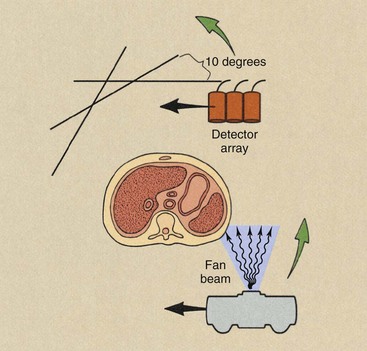
FIGURE 28-4 Second-generation computed tomography imaging systems operated in the translate and rotate mode with a multiple detector array intercepting a fan-shaped x-ray beam.
One disadvantage of the fan beam is the increased radiation intensity that occurs toward the edges of the beam because of body shape. This is compensated for with the use of a “bow tie” filter. These characteristic features of a first- versus a second-generation CT imaging system are shown in Figure 28-5.
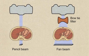
FIGURE 28-5 Profiles of two x-ray beams used in computed tomography (CT) imaging. With the fan-shaped beam of second generation, a bow-tie filter is used to equalize the radiation intensity that reaches the detector array. For first-generation CT, a pencil x-ray beam is used.
The principal advantage of the second-generation CT imaging system was speed. These imaging systems consisted of five to 30 detectors in the detector assembly; therefore, shorter imaging times were possible. Because of the multiple detector array, a single translation resulted in the same number of data points as several translations with a first-generation CT imaging system. Consequently, translations were separated by rotation increments of 5 degrees or more. With a 10-degree rotation increment, only 18 translations would be required for a 180-degree image acquisition.
Second-generation imaging system: translate and rotate, fan beam, detector array, 30-second imaging time.
The principal limitation of second-generation CT imaging systems was examination time. Because of the complex mechanical motion of translation and rotation and the enormous mass involved in the gantry, most units were designed for imaging times of 20 seconds or longer. This limitation was overcome by third-generation CT imaging systems. With these imaging systems, the source and the detector array are rotated about the patient (Figure 28-6). As rotate-only units, third-generation imaging systems can produce an image in less than 1 second.
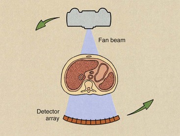
FIGURE 28-6 Third-generation computed tomography imaging systems operate in the rotate-only mode with a fan x-ray beam and a multiple detector array revolving concentrically around the patient.
The third-generation CT imaging system uses a curvilinear array that contains many detectors and a fan beam. The number of detectors and the width of the fan beam—between 30 and 60 degrees—are both substantially larger than for second-generation imaging systems. In third-generation CT imaging systems, the fan beam and the detector array view the entire patient at all times.
The curvilinear detector array produces a constant source-to-detector path length, which is an advantage for good image reconstruction. This feature of the third-generation detector assembly also allows for better x-ray beam collimation and reduces the effect of scatter radiation.
One of the principal disadvantages of third-generation CT imaging systems is the occasional appearance of ring artifacts. If any single detector or bank of detectors malfunctions, the acquired signal or lack thereof results in a ring on the reconstructed image (Figure 28-7). These ring artifacts were troublesome with early third-generation CT imaging systems. Software-corrected image reconstruction algorithms now remove such artifacts.
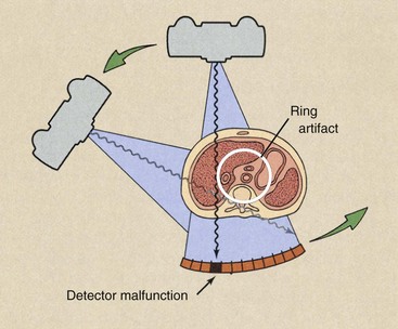
FIGURE 28-7 Ring artifacts can occur in third-generation computed tomography imaging systems because each detector views an annulus (ring) of anatomy during the examination. The malfunction of a single detector can result in the ring artifact.
Third-generation imaging system: rotate and rotate, fan beam, detector array, subsecond imaging time, ring artifacts.
The fourth-generation design for CT imaging systems incorporates a rotate and stationary configuration. The x-ray source rotates, but the detector assembly does not.
Radiation detection is accomplished through a fixed circular array of detectors (Figure 28-8), which contains as many as 4000 individual elements. The x-ray beam is fan shaped with characteristics similar to those of third-generation fan beams. These units are capable of subsecond imaging times, can accommodate variable slice thickness through automatic prepatient collimation, and have the image manipulation capabilities of earlier imaging systems.
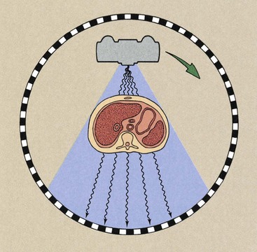
FIGURE 28-8 Fourth-generation computed tomography imaging systems operate with a rotating x-ray source and stationary detectors.
The fixed detector array of fourth-generation CT imaging systems does not result in a constant beam path from the source to all detectors, but it does allow each detector to be calibrated and its signal normalized for each image, as was possible with second-generation imaging systems. Fourth-generation imaging systems were developed because they are free of ring artifacts.
Fourth-generation imaging system: rotate and stationary, fan beam, detector array, subsecond imaging time.
Huge jumps occurred in development between the first and second generations, and even larger developments occurred between the second and third generations. The third-generation version became the de facto baseline model from which later generations were advanced. Today, CT imaging systems are helical, multislice third generation.
Multislice Helical Computed Tomography Imaging Principles
Actually, the gantry motion in multislice helical CT is not like a slinky toy; it just appears that way. Figure 28-9 shows the difference. Figure 28-10 shows the difference between spiral and helical. Many authors, myself included, incorrectly used spiral. See the acknowledgements for a note on this.
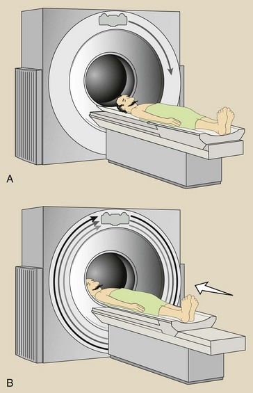
FIGURE 28-9 Movement of the x-ray tube is not helical (A). It just appears that way because the patient moves through the plane of rotation during imaging (B).
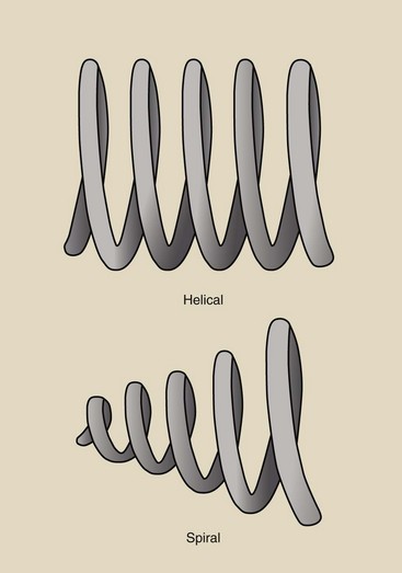
FIGURE 28-10 Illustrating the difference between spiral and helical. We image with helical computed tomography.
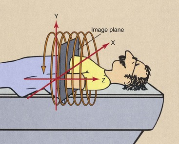
When the examination begins, the x-ray tube rotates continuously. While the x-ray tube is rotating, the couch moves the patient through the plane of the rotating x-ray beam. The x-ray tube is energized continuously, data are collected continuously, and an image then can be reconstructed at any desired z-axis position along the patient (Figure 28-11).
Interpolation Algorithms
Reconstruction of an image at any z-axis position is possible because of a mathematical process called interpolation. Figure 28-12 presents a graphic representation of interpolation and extrapolation. If one wishes to estimate a value between known values, that is interpolation; if one wishes to estimate a value beyond the range of known values, that is extrapolation.
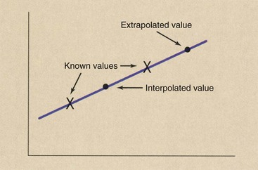
FIGURE 28-12 Interpolation estimates a value between two known values. Extrapolation estimates a value beyond known values.
During helical CT, image data are received continuously, as shown by the data points in Figure 28-13, A. When an image is reconstructed, as in Figure 28-13, B, the plane of the image does not contain enough data for reconstruction. Data in that plane must be estimated by interpolation.
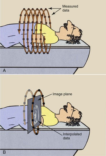
FIGURE 28-13 A, During multislice helical computed tomography, image data are continuously sampled. B, Interpolation of data is performed to reconstruct the image in any transverse plane.
Data interpolation is performed by a special computer program called an interpolation algorithm. The first interpolation algorithms used 360-degree linear interpolation. The plane of the reconstructed image was interpolated from data acquired one revolution apart.
When these images are formatted into sagittal and coronal views, prominent blurring can occur compared with conventional CT reformatted views. The solution to the blurring problem is interpolation of values separated by 180 degrees—half a revolution of the x-ray tube. This results in improved z-axis resolution and greatly improved reformatted sagittal and coronal views.
Pitch
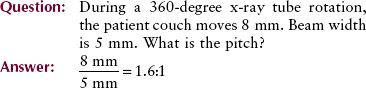
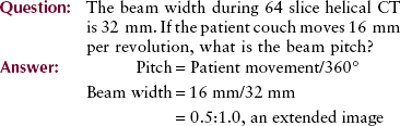
In addition to improved sagittal and coronal reformatted views, 180-degree interpolation algorithms allow imaging at a pitch greater than one. Helical pitch ratio, referred to simply as pitch, is the relationship between patient couch movement and x-ray beam width.
Pitch is expressed as a ratio, such as 0.5 : 1, 1.0 : 1, 1.5 : 1, or 2 : 1. A pitch of 0.5 : 1 results in overlapping images and higher patient radiation dose. A pitch of 2 : 1 results in extended imaging and reduced patient radiation dose.
Increasing pitch to above 1 : 1 increases the volume of tissue that can be imaged at a given time. This is one advantage of multislice helical CT: the ability to image a larger volume of tissue in a single breath-hold. It is particularly helpful in CT angiography, radiation therapy treatment planning, and imaging of uncooperative patients.
The relationship between the volume of tissue imaged and pitch is given as follows:
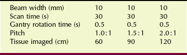
Table 28-1 shows this relationship for a fixed imaging time and a fixed beam width.
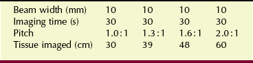
| Question: | How much tissue will be imaged if beam width is set to 8 mm, imaging time is 25 s, and pitch is 1.5 : 1? |
| Answer: | Tissue imaged = 8 mm × 25 s × 1.5 = 300 mm = 30 cm |
What if the gantry rotation time is not 360 degrees in 1 s? In such a situation, the volume of tissue imaged becomes as follows:

If the gantry rotation time is reduced to 0.5 s, Table 28-1 is changed to Table 28-2. With the availability of such fast multislice helical CT, whole-body imaging is now possible within a single breath-hold.
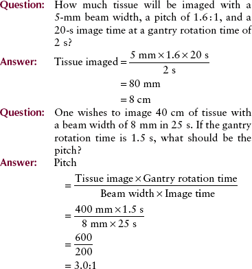
In multislice helical CT, the entire width of the multidetector array (or at least those rows of detectors used for a particular imaging task) intercepts the collimated x-ray beam (Figure 28-14). For example, if all detectors of a 16-slice detector array are used, each of which is 0.5 mm in width, then when the patient couch translates 8 mm, the pitch is 1.0 because the beam width is also 8 mm (Figure 28-15).
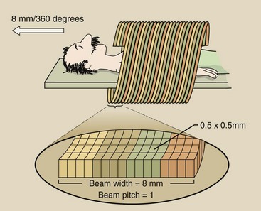
FIGURE 28-14 A 16-detector array, each array element 0.5 mm wide, collimated to an 8 mm beam width results in a pitch of 1.0.
If only the central rows of detectors are used, the x-ray beam width is collimated to 4 mm. Now, if the patient couch translates 8 mm, an extended helix with a beam pitch of 2.0 is observed.
In practice, the pitch for multislice helical CT is usually 1.0. Because multiple slices are obtained and z-axis location and reconstruction width can be selected after imaging, overlapping images are unnecessary.
An exception is CT angiography (CTA), which requires a pitch of less than 1.0 : 1. Because of multislice capability, more slices are acquired per unit time. This results in a much larger volume of imaged tissue.
Unfortunately, when beam pitch exceeds approximately 1.0 : 1, the z-axis resolution is reduced because of a wide section sensitivity profile.
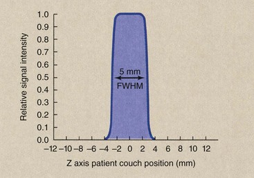
Sensitivity Profile
Consider the sensitivity profile of a 5-mm section obtained with a CT imaging system (Figure 28-16). If properly collimated, it will have a full width at half maximum (FWHM) of 5 mm. The FWHM is the width of the sensitivity. It is also one half of its maximum value.
Imaging System Design
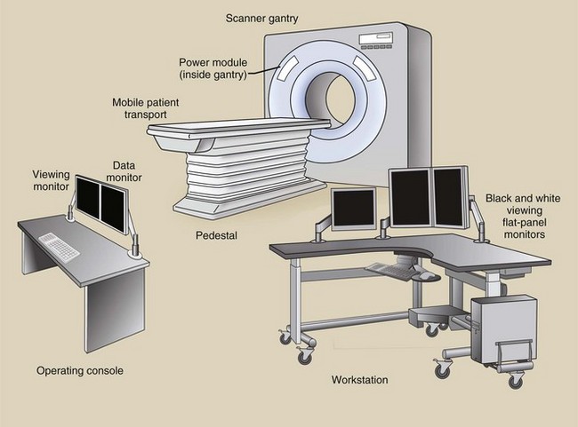
It is convenient to classify the components of a conventional x-ray imaging system into three major subsystems: the operating console, the generator, and the x-ray tube. It is also convenient to identify the three major components of a CT imaging system: the operating console, the computer, and the gantry (Figure 28-17). Each of these major components has several subsystems.
Operating Console
Computed tomography imaging systems can be equipped with two or three consoles. One console is used by the CT radiologic technologist to operate the imaging system. Another console may be available for a technologist to postprocess images to annotate patient data on the image (e.g., hospital identification, name, patient number, age, gender) and to provide identification for each image (e.g., number, technique, couch position). This second monitor also allows the operator to view the resulting image before transferring it to the physician’s viewing console.
A third console may be available for the physician to view the images and manipulate image contrast, size, and general visual appearance. This is in addition to several remote imaging stations.
The operating console contains meters and controls for selection of proper imaging technique factors, for proper mechanical movement of the gantry and the patient couch, and for the use of computer commands that allow image reconstruction and transfer. The physician’s viewing console accepts the reconstructed image from the operator’s console and displays it for viewing and diagnosis.
A typical operating console contains controls and monitors for the various technique factors (Figure 28-18). Operation is usually in excess of 120 kVp, although some recent work supports reducing patient radiation dose by using a lower kVp. The maximum mA is usually 400 mA and is modulated (varied) during imaging according to patient thickness to minimize the patient radiation dose.
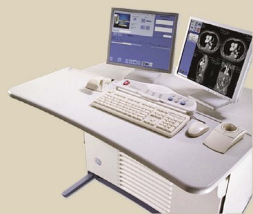
FIGURE 28-18 Operator’s console for a multislice spiral computed tomography imaging system. (Courtesy Reggie Carter, GE Healthcare.)
The thickness of the tissue slice to be imaged also can be adjusted. Nominal thicknesses are 0.5 to 5 mm. Slice thickness is selected from the console by adjustment of the automatic collimator and by selection of various rows of the detector assembly.
Controls also are provided for automatic movement and for indexing of the patient support couch. This allows the operator to program for Z-axis location, tissue volume to be imaged, and spiral pitch.
Physician’s Work Station
This console allows the physician to call up any previous image and manipulate that image to optimize diagnostic information. The manipulative controls provide for contrast and brightness adjustments, magnification techniques, region of interest (ROI) viewing, and use of online computer software packages.
This software may include programs designed to generate plots of CT numbers along any preselected axis, computation of mean and standard. It can also be values in an ROI, subtraction techniques, and planar and volumetric quantitative analysis. Reconstruction of images along coronal, sagittal, and oblique planes is also possible.
The physician’s viewing console is usually remote from the CT suite and is used for postprocessing tasks for all digital images (see Chapter 18). It can also be linked to a picture archiving and communication systems (PACS) network.
Computer
The computer is a unique subsystem of the CT imaging system. Depending on the image format, as many as 250,000 equations must be solved simultaneously; thus, a large computing capacity is required.
At the heart of the computer used in CT are the microprocessor and the primary memory. These determine the time between the end of imaging and the appearance of an image—the reconstruction time. The efficiency of an examination is influenced greatly by reconstruction time, especially when a large number of image slices are involved.
Many CT imaging systems use an array processor instead of a microprocessor for image reconstruction. The array processor does many calculations simultaneously and hence is significantly faster than the microprocessor.
Gantry
The gantry includes the x-ray tube, the detector array, the high-voltage generator, the patient support couch, and the mechanical support for each. These subsystems receive electronic commands from the operating console and transmit data to the computer for image production and postprocessing tasks.
X-ray Tube
X-ray tubes used in multislice helical CT imaging have special requirements. Multislice helical CT places a considerable thermal demand on the x-ray tube. The x-ray tube can be energized up to 60 s continuously. Although some x-ray tubes operate at relatively low tube current, for many, the instantaneous power capacity must be high.
High-speed rotors are used in most for the best heat dissipation. Experience has shown that x-ray tube failure is a principal cause of CT imaging system malfunction and is the principal limitation on sequential imaging frequency.
Focal-spot size is also important in most designs even though the CT image is not based on principles of direct projection imaging. CT imaging systems designed for high spatial resolution imaging incorporate x-ray tubes with a small focal spot.
Multislice helical CT x-ray tubes are very large. They have an anode heat storage capacity of 8 MHU or more. They have anode-cooling rates of approximately 1 MHU per minute because the anode disc has a larger diameter, and it is thicker, resulting in much greater mass.
The limiting characteristics are focal-spot design and heat dissipation. The small focal spot must be especially robust in design. Manufacturers design focal-spot cooling algorithms to predict the focal-spot thermal state and to adjust the mA setting accordingly. The x-ray tube in Figure 28-19 is designed especially for helical CT.
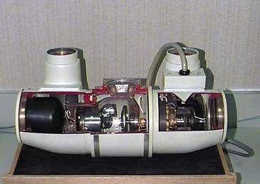
FIGURE 28-19 This x-ray tube is designed especially for spiral computed tomography. It has a 15-cm-diameter disc that is 5 cm thick with an anode heat capacity of 7 MHU. (Courtesy Randy Hood, Philips Medical Systems.)
One company has produced a revolutionary x-ray tube in which the whole insert rotates in a bath of oil during an exposure. The beam of electrons is deflected onto the anode in a process similar to that seen in a cathode ray tube. The result is that it can withstand up to 30 million heat units and cools at a rate of 5 million heat units per minute (see Figure 6-16).
Detector Array
Multislice helical CT imaging systems have multiple detectors in an array that numbers up to tens of thousands (Figure 28-20). Previously, gas-filled detectors were used, but now, all are scintillation, solid state detectors.
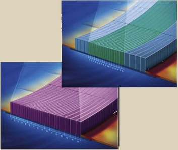
FIGURE 28-20 This multidetector array contains 64 rows of 1824 individual detectors, each 0.6 mm wide (116,736 detectors). (Courtesy Andrew Moehring, GE Healthcare.)
Sodium iodide (NaI) was the crystal used in the earliest imaging systems. This was quickly replaced by bismuth germanate (Bi4Ge3O12 or BGO) and cesium iodide (CsI). Cadmium tungstate (CdWO4) and special ceramics are the current crystals of choice. The concentration of scintillation detectors is an important characteristic of a CT imaging system that affects the spatial resolution of the system.
Scintillation detectors have high x-ray detection efficiency. Approximately 90% of the x-rays incident on the detector are absorbed, and this contributes to the output signal. It is now possible to pack the detectors so that the space between them is nil. Consequently, overall detection efficiency approaches 90%. The efficiency of the x-ray detector array reduces patient radiation doses, allows faster imaging time, and improves image quality by increasing signal-to-noise ratio. Detector array design is especially critical for multislice helical CT.
Collimation
Collimation is required during multislice helical CT imaging for precisely the same reasons as in conventional radiography. Proper collimation reduces patient radiation dose by restricting the volume of tissue irradiated. Even more important is the fact that it improves image contrast by limiting scatter radiation.
In radiography, only one collimator is mounted on the x-ray tube housing. In multislice helical CT imaging, two collimators are used (Figure 28-21).
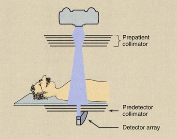
FIGURE 28-21 Multislice helical computed tomography imaging systems incorporate both a prepatient collimator and a predetector collimator.
One collimator is mounted on the x-ray tube housing or adjacent to it. This collimator limits the area of the patient that intercepts the useful beam and thereby determines the patient radiation dose. This prepatient collimator usually consists of several sections, so a nearly parallel x-ray beam results.
The predetector collimator restricts the x-ray beam viewed by the detector array. This collimator reduces the scatter radiation incident on the detector array and, when properly coupled with the prepatient collimator, defines the slice thickness, also called the sensitivity profile. The predetector collimator reduces scatter radiation that reaches the detector array, thereby improving image contrast.
High-Voltage Generator
All multislice helical CT imaging systems operate on high-frequency power. A high-frequency generator is small because the high-voltage step-up transformer is small, so it can be mounted on the rotating gantry.
The design constraints placed on the high-voltage generator are the same as those for the x-ray tube. In a properly designed multislice helical CT imaging system, the two should be matched to maximum capacity. Approximately 50 kW power is necessary.
Patient Positioning and the Support Couch
In addition to supporting the patient comfortably, the patient couch must be constructed of low-Z material, such as carbon fiber, so it does not interfere with x-ray beam transmission and patient imaging. It should be smoothly and accurately motor driven to allow precise patient positioning that is unaffected by the weight of the patient.
When patient couch positioning is not exact, the same tissue can be imaged twice, thus doubling the radiation dose, or it can be missed altogether. The patient couch is indexed automatically, so the operator does not have to enter the examination room between imaging sequences. Such a feature reduces the examination time required for each patient.
Slip-Ring Technology
Slip rings are electromechanical devices that conduct electricity and electrical signals through rings and brushes from a rotating surface onto a fixed surface. One surface is a smooth ring and the other a ring with brushes that sweep the smooth ring (Figure 28-22). Helical CT is made possible by the use of slip-ring technology, which allows the gantry to rotate continuously without interruption.
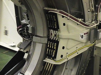
FIGURE 28-22 Slip rings and brushes electrically connect the components on the rotating gantry with the rest of the multislice helical computed tomography imaging system. (Courtesy Terry Williams, Toshiba Medical Systems.)
Early CT imaging was performed with a pause between gantry rotations because high voltage and data cables passed from the gantry. During the pause, the patient couch was moved and the gantry was rewound to a starting position.
In a slip-ring gantry system, power and electrical signals are transmitted through stationary rings within the gantry, thus eliminating the need for electrical cables and making continuous rotation possible.
Brushes that transmit power to the gantry components glide in contact grooves on the stationary slip ring. Composite brushes made of conductive material (e.g., silver graphite alloy) are used as a sliding contact. The rings should last for the life of the imaging system. The brushes have to be replaced every year or so during preventive maintenance.
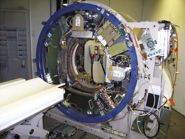
Figure 28-23 shows how compact a rotating gantry must be.
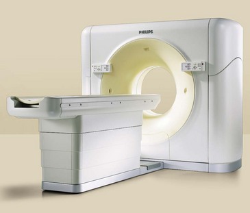
Image Characteristics
The image obtained in CT is different from that obtained in conventional radiography. It is created from data received and is not a projected image. In radiography, x-rays form an image directly on the image receptor. With CT imaging systems, the x-rays form a stored electronic image that is displayed as a matrix of intensities.
Image Matrix
The CT image format consists of many cells, each assigned a number and displayed as an optical density or brightness level on the monitor. The original EMI format consisted of an 80 × 80 matrix for a total of 6400 individual cells of information. Current imaging systems provide matrices of 512 × 512, resulting in 262,144 cells of information.
Each cell of information is a pixel (picture element), and the numerical information contained in each pixel is a CT number, or Hounsfield unit (HU). The pixel is a two-dimensional representation of a corresponding tissue volume (Figure 28-24).
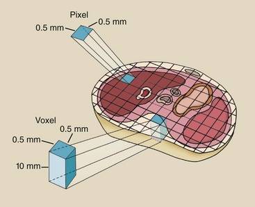
FIGURE 28-24 Each cell in a computed tomography image matrix is a two-dimensional representation (pixel) of a volume of tissue (voxel).
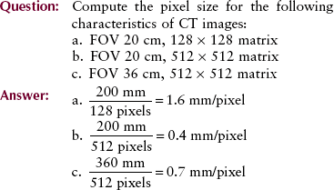
The diameter of image reconstruction is called the field of view (FOV). When the FOV is increased for a fixed matrix size, for example, from 12 cm to 20 cm, the size of each pixel is increased proportionately. When the matrix size is increased for a fixed FOV, for example, 512 × 512 to 1024 × 1024, the pixel size is smaller.
The tissue volume is known as a voxel (volume element), and it is determined by multiplying the pixel size by the thickness of the CT image slice.
Computed Tomography Numbers
Each pixel is displayed on the monitor as a level of brightness. These levels correspond to a range of CT numbers from −1000 to +3000 for each pixel. A CT number of −1000 corresponds to air, and a CT number of +3000 corresponds to dense bone. A CT number of zero indicates water. Table 28-3 shows the CT values for various tissues along with respective x-ray linear attenuation coefficients.
TABLE 28-3
Computed Tomography Number for Various Tissues and X-ray Linear Attenuation Coefficients at Four kVp Techniques
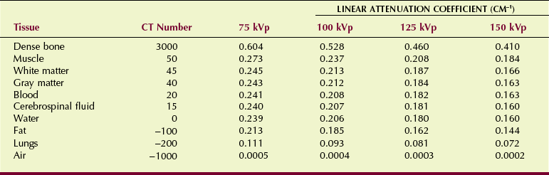
The precise CT number of any given pixel is related to the x-ray attenuation coefficient of the tissue contained in the voxel. As discussed in Chapter 9, the degree of x-ray attenuation is determined by the average energy of the x-ray beam and the effective atomic number of the absorber and is expressed by the attenuation coefficient.
The value of a CT number is given by the following:
 CT Numbers
where µt is the attenuation coefficient of the tissue in the voxel under analysis, µw is the x-ray attenuation coefficient of water, and k is a constant that determines the scale factor for the range of CT numbers.
This equation shows that the CT number for water is always zero because for water, µt = µw, so that µt − µw = 0. For the CT imaging system to operate with precision, detector response must be calibrated continuously so that water is always represented by zero.
Obviously, an enormous amount of information is wasted when the actual dynamic range of the image is 4096 but it is displayed on a monitor and viewed as no more than 32 shades of gray. However, completion of postprocessing with window and level adjustment allows the entire range to be made visible.
Image Reconstruction
The projections acquired by each detector during CT are stored in computer memory. The image is reconstructed from these projections by a process called filtered back projection.
Here, the term filter refers to a mathematical function rather than to a metal filter for the x-ray beam. This process is much too complicated to be discussed here, but a simple example helps to explain how it works.
Imagine a box with two holes cut into each side (Figure 28-25). The box is divided into four cells labeled a, b, c, and d, and a Texas-sized cockroach is found in cell c. If we now cover the box and look through the four sets of holes, we can devise a way of determining precisely in which section the cockroach resides.
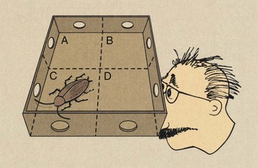
FIGURE 28-25 This four-pixel matrix demonstrates the method for reconstructing a computed tomography image by back projection.
Let “1” represent the presence of the cockroach for each viewing. If one can see through a hole, two empty cells, and the opposite hole, then obviously, the cockroach is not there. We indicate the absence of the cockroach with “0.” The path that is being viewed in Figure 28-25 can be represented symbolically as c + d = 1. Examination of all possible paths shows the following:
The result is four equations for which, if solved simultaneously, the solution is c = 1 and a, b, and d = 0.
In CT, we would have not four cells (pixels) but rather more than 250,000. Consequently, CT image reconstruction requires the solution of more than 250,000 equations simultaneously.
Recently, a more robust reconstruction algorithm, iterative reconstruction, has been introduced. Iterative reconstruction requires more computer capacity but can result in improved contrast resolution at lower patient radiation dose.
Multiplanar Reformation
Multislice helical CT excels in three-dimensional multiplanar reformation (MPR). Transverse images are stacked to form a three-dimensional data set, which can be rendered as an image in several ways. Three three-dimensional MPR algorithms are used most frequently: maximum intensity projection (MIP), shaded surface display (SSD), and shaded volume display (SVD).
Maximum intensity projection reconstructs an image by selecting the highest value pixels along any arbitrary line through the data set and exhibiting only those pixels (Figure 28-26). MIP images are widely used in CTA because they can be reconstructed very quickly.
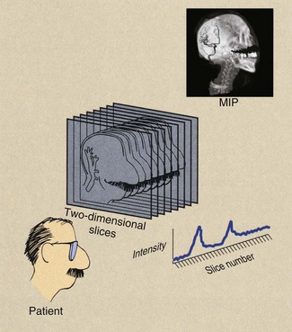
FIGURE 28-26 A maximum intensity projection reconstruction creates a three-dimensional image from multislice two-dimensional data sets. The result is a computed tomographic angiogram.
Only approximately 10% of the three-dimensional data points are used. The result can be a very high-contrast three-dimensional image of contrast-filled vessels (Figure 28-27). On most computer workstations, the image can be rotated to show striking three-dimensional features.
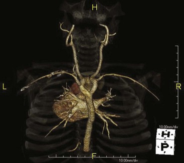
FIGURE 28-27 This carotid computed tomography (CT) scan was reconstructed from a 64-slice spiral CT examination. (Courtesy Lance Blackwell, TeraRecon, Inc.)
Maximum intensity projection is the simplest form of three-dimensional imaging. It provides excellent differentiation of the vasculature from surrounding tissue but lacks vessel depth because superimposed vessels are not displayed. This is accommodated somewhat by image rotation. Small vessels that pass obliquely through a voxel may not be imaged because of partial volume averaging.
Shaded surface display is a computer-aided technique that has been borrowed from computer-aided design and manufacturing applications. It was initially applied to bone imaging and now is used regularly for virtual colonoscopy (Figure 28-28). SSD identifies a narrow range of values as belonging to the object to be imaged and displays that range. The range displayed appears as an organ surface that is determined by operator-selected values.
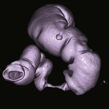
FIGURE 28-28 Shaded surface image obtained during virtual colonoscopy reconstructed from a 64-slice spiral computed tomography data set. (Courtesy Lance Blackwell, TeraRecon, Inc.)
Surface boundaries can be made very distinctive and can provide an image that appears very three-dimensional (Figure 28-29). Such an image is called volume rendered.
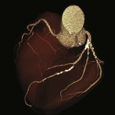
FIGURE 28-29 Volume-rendering display of the heart obtained during cardiac computed tomography angiography (CCTA). This image can be rotated for three-dimensional visualization. (Courtesy Lance Blackwell, TeraRecon, Inc.)
Shaded volume display is very sensitive to the operator-selected pixel range; this can make imaging of actual anatomical structures difficult.
Image Quality
The image quality of conventional radiographs is expressed in terms of spatial resolution, contrast resolution, and noise. These characteristics are relatively easy to describe but somewhat difficult to measure and express quantitatively.
Because CT images are composed of discrete pixel values, image quality is somewhat easier to characterize and quantitate. A number of methods are available for measuring CT image quality, and five principal characteristics are numerically assigned. These include spatial resolution, contrast resolution, noise, linearity, and uniformity.
Spatial Resolution
If one images a regular geometric structure that has a sharp interface, the image at the interface will be somewhat blurred (Figure 28-30). The degree of blurring is a measure of the spatial resolution of the system and is controlled by a number of factors. Because the image of the interface is a visual rendition of pixel values, these values could be analyzed across the interface to arrive at a measure of spatial resolution.
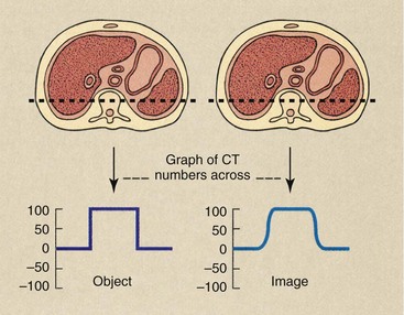
FIGURE 28-30 Computed tomography (CT) examination of an object organ with distinct borders results in an image with somewhat blurred borders. The actual CT number profile of the object is abrupt, but that of the image is smoothed.
The image is somewhat blurred owing to limitations of the CT imaging system; the expected sharp edge of CT values is replaced with a smoothed range of CT values across the interface.
Spatial resolution is a function of pixel size: The smaller the pixel size, the better is the spatial resolution. CT imaging systems allow reconstruction of images after imaging followed by postprocessing tasks; this is a powerful way to affect spatial resolution.
Thinner slice thicknesses also allow better spatial resolution. Anatomy that does not lie totally within a slice thickness may not be resolved, an artifact called partial volume. Therefore, voxel size in CT also affects CT spatial resolution. The design of prepatient and predetector collimation affects the level of scatter radiation and influences spatial resolution by affecting the contrast of the system.
The ability of the CT imaging system to reproduce with accuracy a high-contrast edge is expressed mathematically as the edge response function (ERF). The measured ERF can be transformed into another mathematical expression called the modulation transfer function (MTF). The MTF and its graphic representation are most often cited to express the spatial resolution of a CT imaging system.
Although the MTF is a rather complicated mathematical formulation, its meaning is not too difficult to represent. Return to Chapter 17 and review the concept of MTF. Then consider the series of bar patterns that are imaged by CT (Figure 28-31).
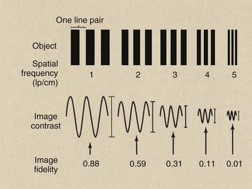
FIGURE 28-31 When a bar pattern of increasing spatial frequency is imaged, the fidelity of the image decreases. The tracing of image contrast reveals the loss of object information.
The spatial frequency for CT imaging systems is expressed often as line pairs per centimeter (lp/cm) instead of line pair per millimeter (lp/mm).
| Question: | How does one convert lp/cm to lp/mm? |
| Answer: | 1 lp/cm = 1 lp/10 mm = 0.1 lp/mm |
A low spatial frequency represents large objects and a high spatial frequency represents small objects.
The image obtained from the low-frequency bar pattern will appear more similar to the object than the image from the high-frequency bar pattern. The loss in faithful reproduction with increasing spatial frequency occurs because of limitations of the imaging system. Characteristics of the CT imaging system that contribute to such image degradation include collimation, detector size and concentration, mechanical and electrical gantry control, and the reconstruction algorithm.
In simplistic terms, the MTF is the ratio of the image to the object as a function of spatial frequency. If the image faithfully represents the object, the MTF of the CT imaging system would have a value of 1. If the image were simply blank and contained no information whatsoever about the object, the MTF would be equal to zero. Intermediate levels of fidelity result in intermediate MTF values.
In Figure 28-32, image fidelity is measured by determining the image contrast along the axis of the image. At a spatial frequency of 1 lp/cm, for instance, the variation in image contrast of the image is 0.88 times that of the object. At 4 lp/cm, it is only 0.11 or 11% that of the object. A graph of this ratio of image contrast to object contrast at each spatial frequency results in an MTF curve (Figure 28-32).
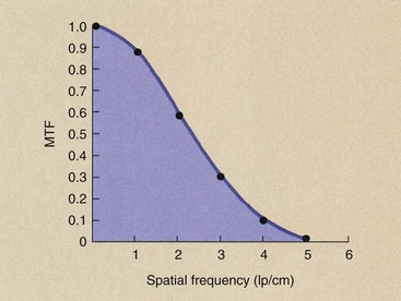
FIGURE 28-32 The modulation transfer function (MTF) is a plot of the image fidelity versus spatial frequency. The six data points plotted here are taken from the analysis of Figure 28-31.
Figure 28-33 shows the MTF for two different CT imaging systems and illustrates how such curves should be interpreted. An MTF curve that extends farther to the right indicates higher spatial resolution, which means the imaging system is better able to reproduce very small objects. An MTF curve that is higher at low spatial frequencies indicates better contrast resolution (Figure 28-34).
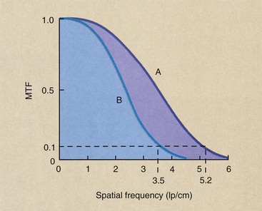
FIGURE 28-33 Modulation transfer function (MTF) curves for two representative computed tomography imaging systems. Imaging system A has higher spatial resolution than imaging system B.
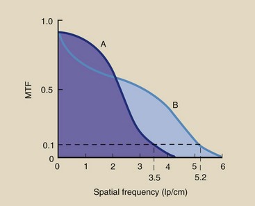
FIGURE 28-34 Imaging system A has better contrast resolution. Imaging system B has better spatial resolution.
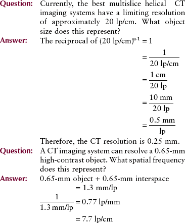
Obviously, MTF is a complex relationship because it relates the imaging capacity of the system for objects of various sizes. Most CT imaging systems are judged by spatial frequency at an MTF equal to 0.1, sometimes called the limiting resolution. As is shown in Figure 28-33, whereas imaging system A has a 0.1 MTF at 5.2 lp/cm, B can manage only 3.5 lp/cm. Therefore, A has better spatial resolution than B.
Although CT image resolution is expressed most often in terms of spatial frequency of the limiting resolution, it is easier to think in terms of the object size that can be reproduced. The absolute object size that can be resolved by a CT imaging system is equal to one-half the reciprocal of the spatial frequency at the limiting resolution.
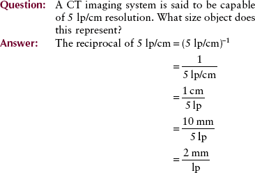
Because a line pair consists of a bar and an interspace of equal width, 2 mm/lp represents a 1-mm object separated by a 1-mm interspace. The system resolution is therefore 1 mm.
Important measures of imaging system performance that can be evaluated with test objects include artifact generation, contrast resolution, and spatial resolution. Figure 28-35
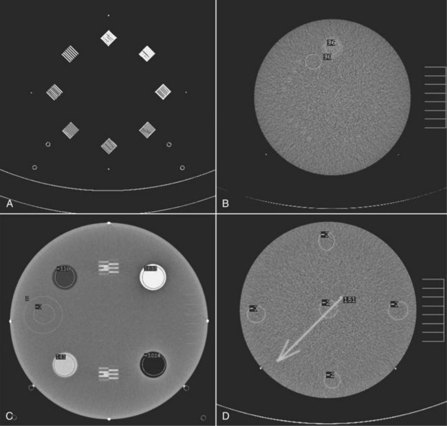
FIGURE 28-35 The phantom for evaluating computed tomography image quality contains test objects designed to measure spatial resolution (A), contrast resolution (B), linearity (C), and other image-quality factors (D). (Courtesy Priscilla Butler, American College of Radiology.)
shows the four test sections of the phantom designed by the Physics Commission of the American College of Radiology (ACR) to evaluate a number of CT image quality factors.
Although MTF and spatial frequency are used to describe CT spatial resolution, no imaging system can do better than the size of a pixel. In terms of line pairs, one line and its interspace require at least two pixels.
Contrast Resolution
The ability to distinguish one soft tissue from another without regard for size or shape is called contrast resolution. This is an area in which multislice helical CT excels.
The absorption of x-rays in tissue is characterized by the x-ray linear attenuation coefficient. This coefficient, as we have seen, is a function of x-ray energy and the atomic number of the tissue. In CT, absorption of x-rays by the patient is determined also by the mass density of the body part.
Consider the situation outlined in Figure 28-36, a fat–muscle–bone structure. Not only are the atomic numbers somewhat different (Z = 6.8, 7.4, and 13.8, respectively), but the mass densities are different (ρ = 0.91, 1.0, and 1.85 g/cm3, respectively). Although these differences are measurable, they are not imaged well on conventional radiography.
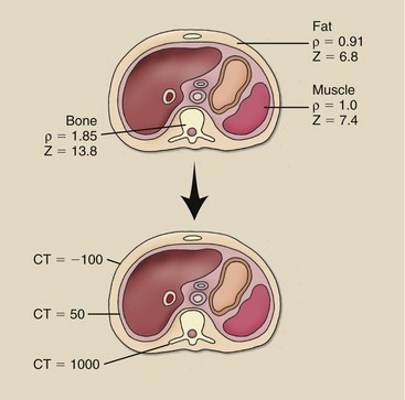
FIGURE 28-36 No large differences are noted in mass density and effective atomic number among tissues, but the differences are greatly amplified by computed tomography imaging.
The CT imaging system is able to amplify these differences in subject contrast so the image contrast is high. The range of CT numbers for these tissues is approximately −
100, 50, and 1000, respectively. This amplified contrast scale allows CT to better resolve adjacent structures that are similar in composition.
The contrast resolution provided by CT is considerably better than that available in radiography principally because of the scatter radiation rejection of the prepatient and predetector collimators. The ability to image low-contrast objects with CT is limited by the size and uniformity of the object and by the noise of the system.
Noise
If a homogeneous medium such as water is imaged, each pixel should have a value of zero. Of course, this never occurs because the contrast resolution of the system is not perfect; therefore, the CT numbers may average zero, but a range of values greater than or less than zero exists.
This variation in CT numbers above or below the average value is the noise of the system. If all pixel values were equal, the noise would be zero.
Noise is the percentage standard deviation of a large number of pixels obtained from a water bath image. It should be clearly understood that noise depends on many factors:
Ultimately, the patient radiation dose, the number of x-rays used by the detector to produce the image, controls noise.
Noise
where xi is each CT value,  is the average of at least 100 values, and n is the number of CT values averaged.
In statistics, noise is called a standard deviation and is symbolized by σ.
Noise appears on the image as graininess. Low-noise images appear very smooth to the eye, and high-noise images appear spotty or blotchy.
Noise should be evaluated daily through imaging of a 20-cm-diameter water bath. All CT imaging systems have the ability to identify an ROI on the digital image and to compute the mean and standard deviation of the CT numbers in that ROI. When the radiologic technologist measures noise, the ROI must encompass at least 100 pixels. Such noise measurements should include five determinations—four on the periphery and one in the center.
Linearity
Computed tomography imaging systems must be calibrated frequently so that water is consistently represented by CT number zero and other tissues by the appropriate CT numbers. A check calibration that can be made daily uses the five-pin performance test object of the American Association of Physicists in Medicine (AAPM) (Figure 28-37). Each of the five pins is made of a different plastic material that has known physical and x-ray attenuation properties and is positioned in a water bath (Table 28-4).
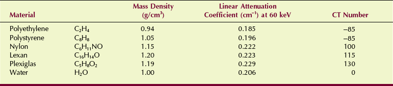
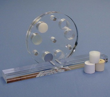
FIGURE 28-37 A version of the five-pin test object designed by the American Association of Physicists in Medicine. The attenuation coefficient for each pin is known precisely, and the computed tomography number is computed. (Courtesy Cardinal Health.)
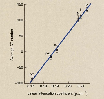
After this test object is imaged, the CT number for each pin should be recorded and its mean value and standard deviation plotted (Figure 28-38). The plot of CT number versus linear attenuation coefficient should be a straight line that passes through CT number 0 for water.
Uniformity
When a uniform object such as a water bath is imaged, each pixel should have the same value because each pixel represents precisely the same object. Furthermore, if the CT imaging system is properly adjusted, that value should be zero. Because the CT imaging system is an extremely complicated electronic mechanical device, however, such precision is not consistently possible. The CT value for water may drift from day to day or even from hour to hour.
At any time that a water bath is imaged, the pixel values should be constant in all regions of the reconstructed image. Such a characteristic is called spatial uniformity.
Spatial uniformity can be tested easily with an internal software package that allows the plotting of CT numbers along any axis of the image as a histogram or as a line graph. If all values of the histogram or line graph are within two standard deviations of the mean value (±2σ), the system is said to exhibit acceptable spatial uniformity. X-ray beam hardening may cause a decrease in CT numbers so that the middle of the image appears darker than the periphery. This is the “cupping” artifact, and it can be clearly demonstrated by imaging the water bath inside a Teflon ring to simulate bone.
Imaging Technique
Multislice helical CT imaging systems have two principal distinguishing features. First, instead of a detector array, multislice helical CT requires several parallel detector arrays that contain thousands of individual detectors (see Figure 28-20). Second, quickly energizing such a large detector array for large-volume imaging requires a very fast large-capacity computer.
After the initial demonstration of dual-slice imaging in the early 1990s, the number of detector arrays have steadily increased to 320 image slices simultaneously that are now available.
A simple approach to multislice helical CT imaging is the use of four detector arrays, each of equal width. This design is shown in Figure 28-39 with a beam pitch of 2.0 : 1—the x-ray beam width is half the patient couch movement. The width of each detector array is 0.5 mm, resulting in four slices, each of 0.5-mm width.
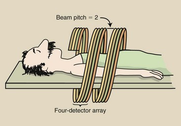
FIGURE 28-39 A four-slice helical computed tomography (CT) scan with a pitch of 2.0 covers eight times the tissue volume of single-slice helical CT.
The design of such a multislice CT imaging system usually allows detected signals from adjacent arrays to be combined to produce two slices of 1-mm width or one slice of 2-mm width (Figure 28-40). Wider slice imaging results in better contrast resolution at the same mA setting because the detected signal is higher.
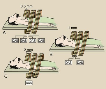
FIGURE 28-40 A four-slice helical computed tomography scan allows changes to be made in slice thickness. A, Four slices of 0.5 mm each. B, Two 0.5-slices can be combined to make two 1-mm slices. C, Four 0.5-mm slices can be combined to make one 2-mm slice. DAS, data acquisition system.
This improvement in contrast resolution is accompanied by a slight reduction in spatial resolution because of increased voxel size. Alternatively, a larger tissue volume can be imaged with original contrast resolution at a reduced mA setting.
This discussion of multislice helical CT has used four slices for simplicity as an example. In fact, multislice helical CT has progressed from 4 to 16, to 64, to 128, to 256, and to 320 in a very short time.
A dual source multislice CT imaging system is shown in Figure 28-41. This system has two x-ray tubes and two detector arrays mounted on the revolving gantry. Imaging speed is its principal advantage; 80 ms imaging is possible.
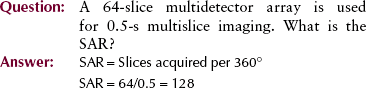
Data Acquisition Rate
Multislice helical CT results in acquisition of multiple slices in the same time previously required for a single slice. The slice acquisition rate (SAR) is one measure of the efficiency of the multislice helical CT imaging system.
The principal advantage of multislice helical CT is that a larger volume of tissue can be imaged. At the limit, it is now possible to image the entire body—from head to toe—in a single breath-hold. Although a volume of tissue is being imaged, this volume is represented by z-axis coverage as follows:
Z-Axis Coverage

where N is the number of slices acquired, R is the rotation time, W is the slice width, T is the imaging time, and B is the pitch.

The advantages and limitations of multislice helical CT are summarized in Table 28-5.
TABLE 28-5
Features of Multislice Helical Computed Tomography
| What | How and Why | |
| Advantages | No motion artifacts | Removes respiratory misregistration |
| Improved lesion detection | Reconstructs at arbitrary z-axis intervals | |
| Reduced partial volume | Reconstructs at overlapping z-axis intervals | |
| Reconstructs smaller than image interval | ||
| Optimized intravenous contrast | Data obtained during peak of enhancement | |
| Reduces volume of contrast agent | ||
| Multiplanar images | Higher-quality reconstruction | |
| Improved patient throughput | Reduces imaging time | |
| Limitations | Increased image noise | Bigger x-ray tubes needed |
| Reduced z-axis resolution | Increases with pitch | |
| Increased processing time | More data and more images needed |
Computed Tomography Quality Control
Computed tomography imaging systems are subject to all the misalignment, miscalibration, and malfunction difficulties of conventional x-ray imaging systems. They have the additional complexities of the multimotional gantry, the interactive console, and the associated computers.
Each of these subsystems increases the risk of drift and instability, which could result in degradation of image quality. Consequently, a dedicated quality control (QC) program is essential for each CT imaging system. Such a program includes daily, weekly, monthly, and annual monitoring in addition to an ongoing preventive maintenance program.
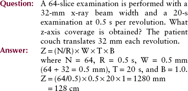
Figure 28-42 shows a popular test object for CT measurements—the ACR CT accreditation phantom. The measurements specified for an annual performance also should be conducted for all new equipment and for all existing equipment after replacement or repair of a major component.
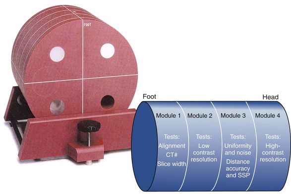
FIGURE 28-42 This computed tomography test object is used to evaluate noise spatial resolution, contrast resolution, slice thickness, linearity, and uniformity. (Courtesy Priscilla Butler, American College of Radiology.)
Noise and Uniformity
A 20-cm water bath should be imaged weekly; the average value for water should be within ±10 HU of zero. Furthermore, uniformity across the image should not vary by more than ±10 HU from the center to the periphery.
Nearly all CT imaging systems easily meet these performance specifications. If a system is used for quantitative CT, however, tighter specifications may be appropriate. When this assessment is performed, one should change one or more of the following: CT scan parameters, slice thickness, reconstruction diameter, or reconstruction algorithm.
Linearity
Linearity is assessed with an image of the AAPM five-pin insert. Analysis of the values of the five pins should show a linear relationship between the Hounsfield unit and electron density. The coefficient of correlation for this linear relationship should be at least 0.96%, or 2 standard deviations.
This assessment should be conducted semiannually. It is particularly important for systems used for quantitative CT, which requires precise determination of the value of tissue in Hounsfield units.
Spatial Resolution
Monitoring of spatial resolution is the most important component of this QC program. Constant spatial resolution ensures proper performance of the detector array, reconstruction electronics, and the mechanical components.
Spatial resolution is assessed by imaging a wire or an edge to obtain the point-spread function or the edge-response function, respectively. These functions then are mathematically transformed to obtain the MTF.
However, determining the MTF requires considerable time and attention. Most medical physicists find it acceptable to image a bar pattern or a hole pattern. Spatial resolution should be assessed semiannually and should be within the manufacturer’s specifications.
Contrast Resolution
Computed tomography excels as an imaging modality because of its superior contrast resolution. The performance specifications of the various CT imaging systems differ from one manufacturer to another and from one model to another, depending on the design of the imaging system. All CT imaging systems should be capable of resolving 5-mm objects at 0.5% contrast.
Contrast resolution should be assessed semiannually. This is done with any of a number of low-contrast test objects with the built-in analytic schemes that are available on all CT imaging systems (Figure 28-43).
Slice Thickness
Slice thickness (sensitivity profile) is measured with the use of a specially designed test object that incorporates a ramp, a spiral, or a step wedge. This assessment should be done semiannually; the slice thickness should be within 1 mm of the intended slice thickness for a thickness of 5 mm or greater. For an intended slice thickness of less than 5 mm, the acceptable tolerance is 0.5 mm.
Couch Incrementation
With automatic maneuvering of the patient through the CT gantry, the patient must be precisely positioned. This evaluation should be done monthly. During a clinical examination with a patient-loaded couch, note the position of the couch at the beginning and at the end of the examination with the use of a tape measure and a straightedge on the couch rails. Compare this with the intended couch movement. It should be within ±2 mm.
Laser Localizer
Most CT imaging systems have internal and/or external laser-localizing lights for patient positioning. The accuracy of these lasers can be determined with any number of specially designed test objects. Their accuracy should be assessed at least semiannually; this is usually done at the same time as the evaluation of couch incrementation.
Patient Radiation Dose
No recommended limits are specified for patient dose during CT examination. Furthermore, dose varies considerably according to scan parameters. High-resolution imaging requires a higher dose.
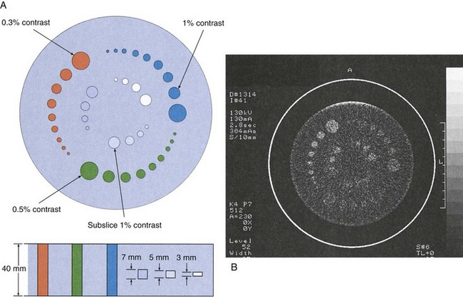
Patient radiation dose is specified as CT dose index or dose-length product and can be monitored with specially designed pencil ionization chambers or thermoluminescent dosimeters. Figure 28-44 shows these measurements in progress. More on patient radiation dose is found in Chapter 37.
Summary
The multislice helical CT imaging system does not record an image as in radiography. The collimated x-ray beam is directed to the patient; the attenuated image-forming x-ray beam is measured by a detector array; the signal from the detector array is analyzed by a computer; the image is reconstructed in the computer; and, finally, the image is displayed on a flat-panel display device.
Multislice helical CT acquires transverse images, which are sections of anatomy that are perpendicular to the long axis of the body. The resultant computer image is an electronic matrix of intensities. Matrix size is usually 512 × 512 pixels. Each pixel contains numeric information called a CT number or a Hounsfield unit. The pixel is a two-dimensional representation of a corresponding tissue volume voxel.
Contrast resolution of the CT imaging system is excellent because of scatter radiation rejection caused by x-ray beam collimation. The ability to image low-contrast anatomy is limited by the noise of the system. System noise is determined by the number of x-rays used by the detector array to produce the image.
Multislice helical CT offers the following advantages over conventional step-and-shoot CT: (1) Motion blur is reduced, so fewer motion artifacts are noted; (2) imaging time is reduced; (3) partial volume artifact is reduced; and (4) a larger volume of tissue can be imaged.
When the examination begins, the x-ray tube rotates continuously, and the patient couch moves through the plane of the rotating beam. The data collected are reconstructed at any desired z-axis position by interpolation.
Pitch is the ratio of patient couch movement to x-ray beam width. Increasing the pitch to above 1 : 1 increases the volume of tissue that can be imaged and at a reduced patient dose.
The need for the x-ray tube to be energized for longer periods demands higher power levels in the spiral CT x-ray tube. Solid state detector arrays with an overall detection efficiency of approximately 90% are preferred.
The volume of tissue imaged is determined by examination time, couch travel, pitch, and beam width. Improvement in z-axis spatial resolution is noted with helical CT because no gaps in data are apparent, and reconstruction images can even overlap. In addition, helical CT excels in three-dimensional MPR.
1. Define or otherwise identify the following:
2. Name the individual who first demonstrated CT in 1970.
3. Explain the term “linear interpolation at 180 degrees.”
4. What are the components in the gantry portion of the multislice helical CT imaging system?
5. What are the special requirements of the x-ray tube as used in multislice helical CT imaging?
6. Write the formula for the multislice helical CT pitch.
7. What is the volume of tissue imaged with beam width thickness of 10 mm, scan time of 30 s, and pitch of 1.6 : 1?
8. Describe the two collimators used in CT imaging.
9. What material makes up the patient support couch?
10. Explain how slip-ring technology contributed to the development of helical CT.
11. What is the voxel size of a CT imaging system with a 320 × 320 matrix size, a 20-cm reconstruction diameter, and a 0.5-cm slice thickness?
12. The volume of tissue imaged on helical CT is determined by which technique selections?
13. Define multiplanar reformation.
14. Explain the mathematics of the multislice helical CT image reconstruction process.
15. What type of high-voltage generator is used for multislice helical CT?
16. A multislice helical CT imaging system can resolve a 0.65-mm high-contrast object. What spatial frequency does this represent?
17. A 10-s multislice helical CT examination is conducted with a 1.5 : 1 pitch and 5-mm beam width. How much tissue is imaged?
18. Why is multislice helical CT pitch greater than 2 : 1 rarely used?
The answers to the Challenge Questions can be found by logging on to our website at http://evolve.elsevier.com.