Evidence about effects of interventions
After reading this chapter, you should be able to:
• Understand more about study designs appropriate for answering questions about effects of interventions
• Generate a structured clinical question about an intervention for a clinical scenario
• Appraise the validity of randomised controlled trials
• Understand how to interpret the results from randomised controlled trials and calculate additional results (such as confidence intervals) where possible
• Describe how evidence about the effects of intervention can be used to inform practice
This chapter focuses on research that can inform us about the effects of interventions. Let us first consider a clinical scenario that will be useful for illustrating the concepts that are the focus of this chapter.
This clinical scenario raises several questions about the interventions that might be effective for reducing falls in people who are at risk of falling. Is balance and strength training effective in reducing the risk of falls? Does providing advice about how to modify a person's home to make it safer prevent falls in people who are at risk of falling? Which of these interventions is most effective, or are both combined more effective than one intervention alone? How cost-effective are multifactorial falls prevention education programs? These are questions that health professionals might ask when making decisions about which interventions will be most effective and will optimise outcomes for their patients.
As we saw in Chapter 1, clinical decisions are made by integrating information from the best available research evidence with information from our patients, the practice context and our clinical experience. Given that one of the most common information needs in clinical practice relates to questions about the effects of interventions, this chapter will begin by reviewing the role of the study design that is used to test intervention effects, before moving on to explaining the process of finding and appraising research evidence about the effects of interventions.
Study designs that can be used for answering questions about the effects of interventions
There are many different study designs that can provide information about the effects of interventions. Some are more convincing than others in terms of the degree of bias that might be in play given the methods used in the study. From Chapter 2, you will recall that bias is any systematic error in collecting and interpreting data. In Chapter 2, we also introduced the concept of hierarchies of evidence. The higher up the hierarchy that a study design is positioned, in the ideal world, the more likely it is that the study design can minimise the impact of bias on the results of the study. That is why randomised controlled trials (sitting second from the top of the hierarchy of evidence for questions about the effects of interventions) are so commonly recommended as the study design that best controls for bias when testing the effectiveness of interventions. Systematic reviews of randomised controlled trials are located above them (at the top of the hierarchy), because these can combine the results of multiple randomised controlled trials. This can potentially provide an even clearer picture about the effectiveness of interventions, providing they are undertaken rigorously. Systematic reviews are explained in more detail in Chapter 12.
One of the best methods for limiting bias in studies that test the effects of interventions is to have a control group.1 A control group is a group of participants in the study who should be as similar in as many ways as possible to the intervention group except that they do not receive the intervention being studied. Let us first have a look at studies that do not use control groups and identify some of the problems that can occur.
Studies that do not use control groups
Uncontrolled studies are studies where the researchers describe what happens when participants are provided with an intervention, but the intervention is not compared with other interventions. Examples of uncontrolled study designs are case reports, case series and before and after studies. These study designs were explained in Chapter 2. The big problem with uncontrolled studies is that when participants are given an intervention and simply followed for a period of time with no comparison against another group, it is impossible to tell how much (if any) of the observed change is due to the effect of the intervention itself or is due to some other factor or explanation. There are some alternative explanations for effects seen in uncontrolled studies, and these need to be kept in mind if you use this type of study to guide your clinical decision making. Some of the forms of bias that commonly occur in uncontrolled studies are described below.
• Volunteer bias. People who volunteer to participate in a study are usually systematically different from those who do not volunteer. They tend to be more motivated and concerned about their health. If this is not controlled for, it is possible that the results can make the intervention appear more favourable (that is, more effective) than it really is. This type of bias can be controlled for by randomly allocating participants, as we shall see later in this chapter.
• Maturation. A participant may change between the time of pre-test (that is, before the intervention is given) and post-test (after the intervention has finished) as a result of maturation. For example, consider that you wanted to measure the improvement in fine motor skills that children in grade 2 of school experienced as a result of a fine-motor-skill intervention program. If you test them again in grade 3, you will not know if the improvements that occurred in fine motor skills happened because of natural development (maturation) or because of the intervention.
• Natural progression. Many diseases and health conditions will naturally improve over time. Improvements that occur in participants may or may not be due to the intervention that was being studied. The participants may have improved on their own with time, not because of the intervention.
• Regression to the mean. This is a statistical trend that occurs in repeated non-random experiments, where participants' results tend to move progressively towards the mean of the behaviour/outcome that is being measured. This does not occur due to maturation or improvement over time, but due to the statistical likelihood of someone with high scores not doing as well when a test is repeated or of someone with low scores being statistically likely to do better when the test is repeated. Suppose, for example, that you used a behavioural test to assess 200 children who had attention deficit hyperactivity disorder and scored their risk of having poor academic outcomes, and that you then provided the 30 children who had the poorest scores with an intensive behavioural regimen and medication. Even if the interventions were not effective, you would still expect to observe some improvement in the children's scores on the behavioural test when it is next given, due to regression to the mean. When outliers are repeatedly measured, subsequent values are less likely to be outliers (that is, they are expected to be closer to the mean value of the whole group). This always happens, and health professionals who do not expect this to occur often attribute any improvement that is observed to the intervention. The best way to deal with the problem of regression to the mean is to randomly allocate participants to either an experimental group or a control group. The regression to the mean effect can only be accounted for by using a control group (which will have the same regression to the mean if the randomisation succeeded and the two groups are similar). How to determine this is explained later in this chapter.
• Placebo effect. This is a well-known type of bias where an improvement in the participants' condition occurs because they expect or believe that the intervention they are receiving will cause an improvement (even though, in reality, the intervention may not be effective at all).
• Hawthorne effect. This is a type of bias that can occur when participants experience improvements not because of the intervention that is being studied, but because of the attention that participants are receiving from being a part of the research process.
• Rosenthal effect. This occurs when participants perform better because they are expected to and, in a sense, this expectation has a similar sort of effect as a self-fulfilling prophecy.
Controlled studies
It should now be clear that having a control group which can be compared with the intervention group in a study is the best way of making sure that bias and extraneous factors that can influence the results of a study are limited. However, it is not as simple as just having a control group as part of the study. The way in which the control group is created can make an enormous difference to how well the study design actually controls for bias.
Non-randomised controlled studies
You will recall from the hierarchy of evidence about the effects of interventions (in Chapter 2) that case-control and cohort studies are located above uncontrolled study designs. This is because they make use of control groups. Cohort studies follow a cohort that has been exposed to a situation or intervention and have a comparison group of people who have not been exposed to the situation of interest (for example, they have not received any intervention). However, because cohort studies are observational studies, the allocation of participants to the intervention and control groups is not under the control of the researcher. It is not possible to tell whether the participants in the intervention and the control groups are similar in terms of all the important factors and, therefore, it is unclear to what extent the exposure (that is, the intervention) might be the reason for the outcome rather than some other factor.
We saw in Chapter 2 that a case-control study is one in which participants with a given disease (or health condition) in a given population (or a representative sample) are identified and are compared with a control group of participants who do not have that disease (or health condition). When a case-control study has been used to answer a question about the effect of an intervention, the ‘cases’ are participants who have been exposed to an intervention and the ‘controls’ are participants who have not. As with cohort studies, because this is an observational study design, the researcher cannot control the assembly of the groups under study (that is, which participants go into which group). Although the controls that are assembled may be similar in many ways to the ‘cases’, it is unlikely that they will be similar with respect to both known and unknown confounders. Chapter 2 explained that confounders are factors that can become confused with the factor of interest (in this case, the intervention that is being studied) and obscure the true results.
In a non-randomised experimental study, the researchers can control the assembly of both experimental and control groups, but the groups are not assembled using random allocation. In non-randomised studies, participants may choose which group they want to be in, or they may be assigned to a group by the researchers. For example, in a non-randomised experimental study that is evaluating the effectiveness of a particular public health intervention (such as an intervention that encourages walking to work) in a community setting, a researcher may assign one town to the experimental condition and another town to the control condition. The difficulty with this approach is that the people in these towns may be systematically different to each other and so confounding factors, rather than the intervention that is being trialled, may be the reason for any difference that is found between the groups at the end of the study.
So not only are control groups essential, but in order to make valid comparisons between groups they must also be as similar as possible at the beginning of a study. This is so that we can say, with some certainty, that any differences found between groups at the end of the study are likely to be due to the factor under study (that is, the intervention), rather than because of bias or confounding. To maximise the similarity between groups at the start of a study, researchers need to control for both known and unknown variables that might influence the results. The best way to achieve this is through randomisation. Non-randomised studies are inherently biased in favour of the intervention that is being studied, which can lead researchers to reach the wrong conclusion about the effectiveness of the intervention.2
Randomised controlled trials
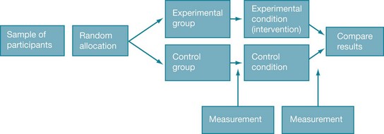
The key feature of randomised controlled trials is that the participants are randomly allocated to either an intervention (experimental) group or a control group. The outcome of interest is measured in participants in both groups before (known as pre-test) and again after (known as post-test) the intervention has been provided. Therefore, any changes that appear in the intervention group pre-test to post-test, but not in the control group, can reasonably be attributed to the intervention. Figure 4.1 shows the basic design of a randomised controlled trial.
You may notice that we keep referring to how randomised controlled trials can be used to evaluate the effectiveness of an intervention. It is worth noting that they can also be used to evaluate the efficacy of an intervention. Efficacy refers to interventions that are tested in ideal circumstances, such as where intervention protocols are very carefully supervised and participant selection is very particular. Effectiveness is an evaluation of an intervention in circumstances that are more like real life, such as where there is a broader range of participants included and a typical clinical level of intervention protocol supervision. In this sense, effectiveness trials are more pragmatic in nature (that is, they are accommodating of typical practices) than are efficacy trials.
There are a number of variations on the basic randomised controlled trial design, which partly depend on the type or combination of control groups used. There are many variations on what the participants in a control group in a randomised controlled trial actually receive. For example, participants may receive no intervention of any kind (a ‘no intervention’ control), or they may receive a placebo, some form of social control or a comparison intervention. In some randomised controlled trials, there are more than two groups. For example, in one study there might be two intervention groups and one control group or, in another study, there might be an intervention group, a placebo group and a ‘no intervention’ group. Randomised crossover studies are a type of randomised controlled trial in which all participants take part in both intervention and control groups, but in random order. For example, in a randomised crossover trial of transdermal fentanyl (a pain medication) and sustained-release oral morphine (another pain medication) for treating chronic non-cancer pain, participants were assigned to one of two intervention groups.3 One group was randomised to four weeks of treatment with sustained-release oral morphine, followed by transdermal fentanyl for four weeks. The second group received the same treatments but in reverse order. A difficulty with crossover trials is that there needs to be a credible wash-out period. That is, the effects of the intervention provided in the first phase must no longer be evident prior to commencing the second phase. In the example we used here, the effect of oral morphine must be cleared prior to the fentanyl being provided.
As we have seen, the advantage of a randomised controlled trial is that any differences found between groups at the end of the study are likely to be due to the intervention rather than to extraneous factors. But the extent to which these differences can be attributed to the intervention is also dependent on some of the specific design features that were used in the trial, and these deserve close attention. The rest of this chapter will look at randomised controlled trials in more depth within the context of the clinical scenario that was presented at the beginning of this chapter. In this scenario you are a health professional who is working in a small group at a community health centre and you are looking for research regarding the effectiveness of falls prevention programs. To locate relevant research, you start by focusing on what it is that you specifically want to know about.
How to structure a question about the effect of an intervention
In Chapter 2, you learnt how to structure clinical questions using the PICO format: Patient/Problem/Population, Intervention/Issue, Comparison (if relevant) and Outcomes.
In our falls clinical scenario, the population that we are interested in is elderly people who live in the community who fall. We know from our clinical experience that people who have had falls in the past are at risk of falling again, so it makes sense to target our search for interventions aimed at people who are either ‘at risk’ of falling and/or have a history of falling.
The intervention that we think could most readily be delivered in our setting would be a falls prevention education group which targets multiple risk factors for falling and incorporates exercise. Are we interested in a comparison intervention? While we could compare the effectiveness of one type of intervention with another, for this scenario it is probably more useful to start by first thinking about whether the intervention is effective. To do this we would need to compare the intervention to either a placebo (a concept we will discuss later) or to usual care.
There are a number of outcomes that we could consider important for people who fall. The most obvious outcome of interest is a reduction in the number of falls. However, we could also look for interventions that consider the factors contributing to falls, such as balance problems or, in our scenario, a person's confidence (or self-efficacy) to undertake actions that will prevent them from falling.
How to find evidence to answer questions about the effects of an intervention
Our clinical scenario question is a question about the effectiveness of an intervention to prevent falls and to improve self-efficacy. You can use the hierarchy of evidence for this type of question as your guide to know which type of study you are looking for and where to start searching. In this case, you are looking for a systematic review of randomised controlled trials. If there is no relevant systematic review, you should next look for a randomised controlled trial. If no relevant randomised controlled trials are available, you would then need to look for the next best available type of research, as indicated by the hierarchy of evidence for this question type shown in Chapter 2.
As we saw in Chapter 3, the best source of systematic reviews of randomised controlled trials is the Cochrane Database of Systematic Reviews, so this would be the logical place to start searching. The Cochrane Library also contains the Cochrane Central Register of Controlled Trials, which includes a large collection of citations of randomised controlled trials. If you are looking for randomised controlled trials specifically in the rehabilitation field, two other databases that you could consider searching for this topic are PEDro (www.pedro.org.au) or OTseeker (www.otseeker.com). These databases were explained in Chapter 3. One of their advantages is that they have already evaluated the risk of bias that might be of issue in the randomised controlled trials that they index.
Once you have found a research article that you are interested in, it is important to critically appraise it. That is, you need to examine the research closely to determine whether and how it might inform your clinical practice. As we saw in Chapter 1, to critically appraise research, there are three main aspects to consider: (1) its internal validity (in particular, the risk of bias); (2) its impact (the size and importance of any effect found); and (3) whether or how the evidence might be applicable to your patient or clinical practice.
Is this evidence likely to be biased?
In this chapter we will discuss six criteria that are commonly used for appraising the potential risk of bias in a randomised controlled trial. These six criteria are summarised in Box 4.1 and can be found in the Users' guides to the medical literature5 and in many appraisal checklists such as the Critical Appraisal Skills Program (CASP) checklist and the PEDro scale.6 A number of studies have demonstrated that estimates of treatment effects may be distorted in trials that do not adequately address these issues.7,8 As you work through each of these criteria when appraising an article, it is important to consider the direction of the bias (that is, is it in favour of the intervention or the control group?) as well as its magnitude. As we pointed out in Chapter 1, all research has flaws. However, we do not just want to know what the flaws might be, but whether and how they might influence the results of a study.
Was the assignment of participants to groups randomised?
Randomised controlled trials, by definition, randomise participants to either the experimental or the control condition. The basic principle of randomisation is that each participant has an equal chance of being assigned to any group, such that any difference between the groups at the beginning of the trial can be assumed to be due to chance. The main benefit of randomisation is related to the idea that, this way, both known and unknown participant characteristics should be evenly distributed between the intervention and control groups. Therefore, any differences between groups that are found at the end of the study are likely to be because of the intervention.9
Random allocation is best done using a random numbers table which can be computer-generated. Sometimes it is done by tossing a coin or ‘pulling a number out of a hat’. Additionally, there are different randomisation designs that can be used and you should be aware of them. Researchers may choose to use some form of restriction, such as blocking or stratification, when allocating participants to groups in order to create a greater balance between the groups at baseline in known characteristics.10 Different randomisation designs are summarised below.
• Simple randomisation: involves randomisation of individuals to the experimental or the control condition.
• Cluster randomisation: involves random allocation of intact clusters of individuals rather than individuals (for example, randomisation of schools, towns, clinics or general practices).
• Stratified randomisation: in this design, participants are matched and randomly allocated to groups. This method ensures that potentially confounding factors such as age, gender or disease severity are balanced between groups. For example, in a trial that involves people who have had a stroke, participants might be stratified according to their initial stroke severity as belonging to a ‘mild’, ‘moderate’ or ‘severe’ stratum. This way, when randomisation to study groups occurs researchers can ensure that, within each stratum, there are equal numbers of participants in the intervention and control groups.
• Block randomisation: in this design, participants who are similar are grouped into ‘blocks’ and are then assigned to the experimental or control conditions within each block. Block randomisation often uses stratification. An example of block randomisation can be seen in a randomised controlled study of a community-based parenting education intervention program designed to increase the use of preventive paediatric healthcare services among low-income, minority mothers.11 Two hundred and eighty-six mother–infant dyads recruited from four different sites in Washington DC were assigned to either the standard social services (control) group or the intervention group. To ensure that there were comparable numbers within each group across the four sites, site-specific block randomisation was used. By using block randomisation, selection bias due to demographic differences across the four sites was avoided.
Was the allocation sequence concealed?
As we have seen, the big benefit of a randomised controlled trial over other study designs is the fact that participants are randomly allocated to the study groups. However, the benefits of randomisation can be undone if the allocation sequence is manipulated or interfered with in any way. As strange as this might seem, a health professional who wants their patient to receive the intervention being evaluated may swap their patient's group assignment so that their patient receives the intervention being studied. Similarly, if the person who recruits participants to a study knows which condition the participants are to be assigned to, this could influence their decision about whether or not to enrol them in the study. This is why assigning participants to study groups using alternation methods, such as every second person who comes into the clinic, or assigning participants by methods such as date of birth is problematic because the randomisation sequence is known to the people involved.9
Knowledge about which group a participant will be allocated to if they are recruited into a study can lead to the selective assignment of participants, and thus introduce bias into the trial. This knowledge can result in manipulation of either the sequence of groups that participants are to be allocated to or the sequence of participants to be enrolled. Either way, this is a problem. This problem can be dealt with by concealing the allocation sequence from the people who are responsible for enrolling patients into a trial or from those who assign participants to groups, until the moment of assignment.12 Allocation can be concealed by having the randomisation sequence administered by someone who is ‘off-site’ or at a location away from where people are being enrolled into the study. Another way to conceal allocation is by having the group allocation placed in sealed, opaque envelopes. Opaque envelopes are used so that the group allocation cannot be seen if the envelope is held up to the light! The envelope is not to be opened until the patient has been enrolled into the trial (and is therefore now a participant in the study).
Hopefully, the article that you are appraising will clearly state that allocation was concealed, or that it was done by an independent or off-site person or that sealed opaque envelopes were used. Unfortunately, though, many studies do not give any indication about whether allocation was concealed,13,14 so you are often left wondering about this, which is frustrating when you are trying to appraise a study. It is possible that some of these studies did use concealed allocation, but you cannot tell this from reading the article.
Were the groups similar at the baseline or start of the trial?
One of the principal aims of randomisation is to ensure that the groups are similar at the start of the trial in all respects, except for whether they received the experimental condition (that is, the intervention of interest) or not. However, the use of randomisation does not guarantee that the groups will have similar known baseline characteristics. This is particularly the case if there is a small sample size. Authors of a research article will usually provide data in the article about the baseline characteristics of both groups. This allows readers to make up their own minds as to whether the balance between important prognostic factors (variables that have the potential for influencing outcomes) is sufficient at the start of the trial. Consider, for example, a study about the effectiveness of acupuncture for reducing pain from migraines compared with sham acupuncture. If the participants who were allocated to the acupuncture group had less severe or less chronic pain at the start of the study than the participants who were allocated to the sham acupuncture group, any differences in pain levels that were seen at the end of the study might be the result of that initial difference and not the acupuncture that was provided.
Differences between the groups that are present at baseline after randomisation have occurred due to chance and, therefore, determining whether these differences are statistically significant by using p values is not an appropriate way of assessing such differences.15 That is, rather than using the p value that is often reported in studies, it is important to examine these differences by comparing means or proportions visually. The extent to which you might be concerned about a baseline difference between the groups depends on how large a difference it is and whether it is a key prognostic variable, both of which require some clinical judgment. The stronger the relationship between the characteristic and the outcome of interest, the more the differences between groups will weaken the strength of any inference about efficacy.5 For example, consider a study that is investigating the effectiveness of group therapy in improving communication for people who have chronic aphasia following stroke compared with usual care. Typically, such a study would measure and report a wide range of variables at baseline (that is, prior to the intervention) such as participants' age, gender, education level, place of residence, time since stroke, severity of aphasia, side of stroke and so on. Some of these variables are more likely to influence communication outcomes than others. The key question to consider is: are any differences in key prognostic variables between the groups large enough that they may have influenced the outcome(s)? Hopefully, if differences are evident the researchers will have corrected for this in the data analysis process.
As a reader (and critical appraiser) of research articles, it is important that you are able to see data for key characteristics that may be of prognostic value in both groups. Many articles will present such data in a table, with the data for the intervention group presented in one column and the data for the control group in another. This enables you to easily compare how similar the groups are for these variables. As well as presenting baseline data about key socio-demographic characteristics (for example, age and gender), articles should also report data about important measures of the severity of the condition (if that is relevant to the study—most times it is) so that you can see whether the groups were also similar in this respect. For example, in a study that involves participants who have had a stroke, the article may present data about the initial stroke severity of participants, as this variable has the potential to influence how participants respond to an intervention. In most cases, socio-demographic variables alone are not sufficient to determine baseline similarity.
One other area of baseline data that articles should report is the key outcome(s) of the study (that is, the pre-test measurement(s)). Let us consider the example presented earlier of people receiving group communication treatment for aphasia to illustrate why this is important. Although such an article would typically provide information about socio-demographic variables and clinical variables (such as severity of aphasia, type of stroke and side of stroke), having information about participants' initial (that is, pre-test) scores on the communication outcome measure that the study used would be helpful for considering baseline similarity. This is because, logically, participants' pre-test scores on a communication measure are likely to be a key prognostic factor for the main outcome of the study, which is communication ability.
When appraising an article, if you do conclude that there are baseline differences between the groups that are likely to be big enough to be of concern, hopefully the researchers will have statistically adjusted for these in the analysis. If they have not, you will need to try to take this into account when interpreting the study.
Were participants, health professionals and study personnel ‘blind’ to group allocation?
People involved with a trial, whether they be the participants, the treating health professionals or the study personnel, usually have a belief or expectation about what effect the experimental condition will or will not have. This conscious or unconscious expectation can influence their behaviour, which in turn can affect the results of the study. This is particularly problematic if they know which condition (experimental or control) the participant is receiving. Blinding (also known as masking) is a technique that is used to prevent participants, health professionals and study personnel from knowing which group the participant was assigned to so that they will not be influenced by that knowledge.10
In many studies, it is difficult to achieve blinding. Blinding means more than just keeping the name of the intervention hidden. The experimental and control conditions need to be indistinguishable. This is because even if they are not informed about the nature of the experimental or control conditions (which, for ethical reasons, they usually are) when they sign informed consent forms, participants can often work out which group they are in. Whereas pharmaceutical trials can use placebo medication to prevent participants and health professionals from knowing who has received the active intervention, blinding of participants and the health professionals who are providing the intervention is very difficult (and often impossible) in many non-pharmaceutical trials. We will now look a little more closely at why it is important to blind participants, health professionals and study personnel to group allocation.
A participant's knowledge of their treatment status (that is, if they know whether they are receiving the intervention that is being evaluated or not) may consciously or unconsciously influence their performance during the intervention or their reporting of outcomes. For example, if a participant was keen to receive the intervention that was being studied and they were instead randomised to the control group, they may be disappointed and their feelings about this might be reflected in their outcome assessments, particularly if the outcomes being measured are subjective in nature (for example, pain, quality of life or satisfaction). Conversely, if a participant knows or suspects that they are in the intervention group, they may be more positive about their outcomes (such as exaggerating the level of improvement that they have experienced) when they report them, as they wish to be a ‘polite patient’ and are grateful for receiving the intervention.16
The health professionals who provide the intervention often have a view about the effectiveness of interventions, and this can influence the way they interact with the study participants and the way they deliver the intervention. This in turn can influence how committed they are to providing the intervention in a reliable and enthusiastic manner, affecting participants' compliance to the intervention and participants' responses on outcome measures. For example, if a health professional believes strongly in the value of the intervention that is being studied, they may be very enthusiastic and diligent in their delivery of the intervention, which may in turn influence how participants respond to this intervention. It is easy to see how a health professional's enthusiasm (or lack of) could influence outcomes. Obviously some interventions (such as medications) are not able to be influenced easily by the way in which they are provided, but for many other interventions (such as rehabilitation techniques provided by therapists), this can be an issue.
Study personnel who are responsible for measuring outcomes (the assessors) and who are aware of whether the participant is receiving the experimental or control condition may provide different interpretations of marginal findings or differential encouragement during performance tests, either of which can distort results. For example, if an assessor knows that a participant is in the intervention group, they might be a little more generous when scoring a participant's performance on a task than they would be if they thought that the participant was in the control group. Studies should aim to use blinded assessors to prevent measurement bias from occurring. This can be done by ensuring that the assessor who measures the outcomes at baseline and at follow-up is unaware of the participant's group assignment. Sometimes this is referred to as the use of an independent assessor. The more objective the outcome that is being assessed, the less critical this issue becomes. However, there are not many truly objective outcome measures, as even measures that appear to be reasonably objective (for example, measuring muscle strength manually or functional ability) have a subjective component and, as such, can be susceptible to measurement bias. Therefore, where it is at all possible, studies should try to ensure that the people who are assessing participants' outcomes are blinded. Ideally, studies should also check and report on the success of blinding assessors and, where this information is not provided, you may wish to reasonably speculate about whether or not the outcome assessor was actually blinded as claimed.
However, there is a common situation that occurs, particularly in many trials in which non-pharmaceutical interventions are being tested, that makes assessor blinding not possible to achieve. If the participant is aware of their group assignment, then the assessment cannot be considered to be blinded. For example, consider the outcome measure of pain that is assessed using a visual analogue scale. The participant has to complete the assessment themselves due to the subjective nature of the symptom experience. In this situation, the participant is really the assessor and, if the participant is not blind to which study group they are in, then the assessor is also not blind to group allocation. Research articles often state that the outcome assessors were blind to group allocation. Most articles measure more than one outcome and often a combination of objective and subjective outcome measures are used. So, while this statement may be true for objective outcomes, if the article involved outcomes that were assessed by participant self-report and the participants were not blinded, you cannot consider that these subjective outcomes were measured by a blinded assessor.
Were all participants who entered the trial properly accounted for at its conclusion, and how complete was follow-up?
In randomised controlled trials, it is common to have missing data at follow-up. There are many reasons why data may be missing. For example, some questionnaires may not have been fully completed by participants, some participants may have decided to leave the study or some participants may have moved house and cannot be located at the time of the follow-up assessment. How much of a problem this is for the study, with respect to the bias that is consequently introduced, depends on why participants left the study and how many left the study.
It is therefore helpful to know whether all the participants who entered the trial were properly accounted for. In other words, we want to know what happened to them. Could the reason that they dropped out of the study have affected the results? This may be the case, for example, if they left the study because the intervention was making them worse or causing adverse side effects. If this was the case, this might make the intervention look more effective than it really was. Did they leave the study simply because they changed jobs and moved away, or was the reason that they dropped out related to the study or to their health? For example, it may not be possible to obtain data from participants at follow-up measurement points because they became unwell, or maybe because they improved, and no longer wanted to participate. Hopefully, you can now see why it is important to know why there are missing data for some participants.
The more participants who are ‘lost to follow-up’, the more the trial may be at risk of bias because participants that leave the study are likely to have different prognoses from those who stay in the study. It has been suggested that ‘readers can decide for themselves when the loss to follow-up is excessive by assuming, in positive trials (that is, trials that showed that the intervention was effective), that all participants lost from the treatment group did badly, and that all lost from the control group did well, and then recalculating the outcomes under these assumptions. If the conclusions of the trial do not change, then the loss to follow-up was not excessive. If the conclusions would change, the strength of inference is weakened (that is, less confidence can be placed in the study results)’.5
When large numbers of participants leave a study, the potential for bias is enhanced. Various authors suggest that if more than 15–20% of participants leave the study (with no data available for them), then the results should be considered with much greater caution.16,17 Therefore, you are looking for a study to have a minimum follow-up rate of at least 80–85%. To calculate the loss to follow-up, you just need to divide the number of participants included in the analysis at the time point of interest (such as the 6-month follow-up) by the number of participants who were originally randomised into the study groups. This gives the percentage of participants who were followed up. In some articles it is straightforward to find the necessary data that you need to calculate this, particularly if the article has provided a flow diagram (see Figure 4.2). It is highly recommended that trials do this, and this is explained more fully later in the chapter when the recommended reporting of a randomised controlled trial is discussed. In other articles, this information can be obtained from the text, typically in the results section. In some articles, the only place to locate information about the number of participants who remain in the groups at a particular time point is from the column headers in a results table. And finally, in some articles, despite all of your best hunting efforts, there may be no information about the number of participants who were retained in the study. This may mean that there were no participants lost to follow-up (which is highly unlikely, as at least some participants are lost to follow-up in most studies) or the authors of the article did not report the loss of participants that occurred. Either way, as you cannot determine how complete the follow-up was, you should be suspicious of the study and consider the results to be potentially biased.
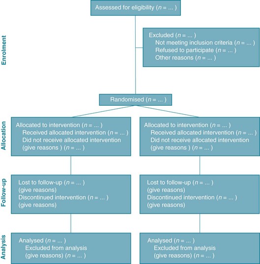
Figure 4.2 CONSORT flow diagram. From Schulz K et al, CONSORT 2010 statement: updated guidelines for reporting parallel-group randomised trials. BMJ 2010; 340:c332;18 reproduced with permission from BMJ Publishing Group Ltd.
It is worth noting that where there is loss to follow-up in both the intervention and the control groups and the reasons for these losses are both known and similar between these groups, it is less likely that bias will be problematic.19 When the reasons why participants leave the study are unknown, or when they are known to be different between the groups and potentially prognostically relevant, you should be more suspicious about the validity of the study. That is why it is important to consider the reasons for loss to follow-up and whether the number of participants lost to follow-up was approximately the same for both of the study groups, as well as the actual percentage of participants who were lost to follow-up.
Were participants analysed in the groups to which they were randomised using intention-to-treat analysis?
The final criterion for assessing risk of bias that we will address in this chapter is whether or not data from all participants were analysed in the groups to which participants were initially randomised, regardless of whether they ended up receiving the treatment. This analysis principle is referred to as intention-to-treat analysis. In other words, participants should be analysed in the group that corresponds to how they were intended to be treated, not how they were actually treated.
It is important that an intention-to-treat analysis is performed, because study participants may not always receive the intervention or control condition as it was allocated (that is, intended to be received). In general, participants may not receive the intervention (even though they were allocated to the intervention group) because they are either unwell or unmotivated, or for other reasons related to prognosis.5 For example, in a study that is evaluating the effect of a medication, some participants in the intervention group may forget to take the medication and therefore do not actually receive the intervention as intended. In a study that is evaluating the effects of a home-based exercise program, some of the participants in the intervention group may not practise any of the exercises that are part of the intervention because they are not very motivated. Likewise, in a study that is evaluating a series of small-group education sessions for people who have had a heart attack, some participants in the intervention group may decide not to attend some or all education sessions because they feel unwell. From these examples, you can see that even though these participants were in the intervention group of these studies, they did not actually receive the intervention (either at all or only partly). It may be tempting for the researchers who are conducting these studies to analyse the data from these participants as if they were in the control group instead. However, doing this would increase the numbers in the control group who were either unmotivated or unwell. This would make the intervention appear more effective than it actually is because there would be a greater number of participants in the control group who were likely to have unfavourable outcomes. It may also be tempting for researchers to discard the results from participants who did not receive the intervention (or control condition) as was intended. This is also an unsuitable way of dealing with this issue, as these participants would then be considered as lost to follow-up and we saw in the previous criterion why it is important that as few participants as possible are lost to follow-up.
For the sake of completeness, it is important to point out that it is not only participants who are allocated to the intervention group but do not receive the intervention that we should think about. The opposite can also happen. Participants who are allocated to the control group can inadvertently end up receiving the intervention. Again, intention-to-treat analysis should be used and these participants should still be analysed as part of the control group.
The value of intention-to-treat analysis is that it preserves the value of randomisation. It helps to ensure that prognostic factors that we know about, and those that we do not know about, will still be, on average, equally distributed between the groups. Because of this, any effect that we see, such as improvement in participants' outcomes, is most likely to be because of the intervention rather than unrelated factors.
The difficulty in carrying out a true intention-to-treat analysis is that the data for all participants is needed. However, as we saw in the previous criterion about follow-up of participants, this is unrealistic to expect and most studies have missing data. There is currently no real agreement about the best way to deal with such missing data (probably because there is no ideal way), but researchers may sometimes estimate or impute data.20 Data imputation is a statistical procedure that substitutes missing data in a data file with estimated data. Other studies may simply report that they have carried out an intention-to-treat analysis or that participants received the experimental or control conditions as allocated without providing details of what was actually done or how missing data were dealt with. In this case, as the reader of the article, you may choose to accept this at face value or to remain sceptical about how this issue was dealt with, depending on what other clues are available in the study report.
The role of chance
So far in this chapter we have considered the potential for bias in randomised controlled trials. Another aspect that is important to consider is the possibility that the play of chance might be an alternative explanation for the findings. So, a further question that you may wish to consider when appraising a randomised controlled trial is: did the study report a power calculation that might indicate what sample size would be necessary for the study to detect an effect if the effect actually exists? As we saw in Chapter 2, having an adequate sample size is important so that the study can avoid a type II error occurring. You may remember that a type II error is the failure to find and report a relationship when a relationship actually exists.21
Completeness of reporting of randomised controlled trials
As we have seen in many places throughout this chapter, it can often be difficult for readers of research studies to know whether a study has or has not met some of the requirements to be considered a well-designed and well-conducted randomised controlled trial that is relatively free of bias. To help overcome this problem and aid in the critical appraisal and interpretation of trials, an evidence-based initiative known as the CONSORT (Consolidated Standards of Reporting Trials) statement12,18 has been developed to guide authors in how to completely report the details of a randomised controlled trial. The CONSORT statement is considered an evolving document and, at the time of writing, it consisted of a 22-item checklist and a flow diagram (see Figure 4.2). Full details are available at www.consort-statement.org. The CONSORT statement is also used by reviewers of articles when the articles are being considered for publication, and many journals now insist that articles about randomised controlled trials follow the CONSORT statement. This is helping to improve the quality of reporting of trials but, as this is a recent requirement, many older articles do not contain all of the information that you need to know.
After determining that an article about the effects of an intervention that you have been appraising appears to be reasonably free of bias, you then proceed to looking at the importance of the results.
Understanding results
One of the fundamental concepts that you need to keep in mind when trying to make sense of the results of a randomised controlled trial is that clinical trials provide us with an estimate of the average effects of an intervention. Not every participant in the intervention group of a randomised controlled trial is going to benefit from the intervention that is being studied—some may benefit a lot, some may benefit a little, some may experience no change and some may even be worse (a little or a lot) as a result of receiving the intervention. The results from all participants are combined and the average effect of the intervention is what is reported.
Before getting into the details about how to interpret the results of a randomised controlled trial, the first thing that you need to look at is whether you are dealing with continuous or dichotomous data:
• Variables with continuous data can take any value along a continuum within a defined range. Examples of continuous variables are age, range of motion in a joint, walking speed and score on a visual analogue scale.
• Variables with dichotomous data have only two possible values. For example, male/female, satisfied/not satisfied with treatment, and hip fracture/no hip fracture.
The way that you make sense of the results of a randomised controlled trial depends on whether you are dealing with outcomes that were continuous or dichotomous. We will look at continuous data first. However, regardless of whether the results of the study were measured using continuous or dichotomous outcomes, we will be looking at how to answer two main questions:
Continuous outcomes—size of the intervention effect
When you are trying to work out how much of a difference the intervention made, you are trying to determine the size of the intervention effect. When you are dealing with continuous data, this is often quite a straightforward process.
Many articles will already have done this for you and will report the difference. In other articles, you will have to do this simple calculation yourself.
Let us consider an example. In a randomised controlled trial22 that evaluated the efficacy of a self-management program for people with knee osteoarthritis in addition to usual care, compared with usual care, one of the main outcome measures was pain, which was measured using a 0–10 cm visual analogue scale with 0 representing ‘no pain at all’ and 10 representing ‘the worst pain imaginable’. At the 3-month follow-up, the mean reduction in knee pain was 0.67 cm (standard deviation [SD] = 2.10) in the intervention group and 0.01 cm (SD = 2.00) in the control group. This difference was statistically significant (p = 0.023). You can calculate the intervention effect size (difference in mean change between the groups) as: 0.67 cm minus 0.01 cm = 0.66 cm.
Note that in this study, the authors reported the mean improvement (reduction in pain) scores at the 3-month follow-up (that is, the change in pain from baseline to the 3-month follow-up). Some studies report change scores; other studies report end scores (which are the scores at the end of the intervention period). Regardless of whether change scores or end scores are reported, the method of calculating the size of the intervention effect is the same. When dealing with change scores, it becomes the difference of the mean change between the intervention and control groups that you need.
Clinical significance
Once you know the size of the intervention effect, you need to decide whether this result is clinically significant. As we saw in Chapter 2, just because a study finds a statistically significant result it does not mean that the result is clinically significant. Deciding whether a result is clinically significant requires your judgment (and, ideally, your patient's, too) on whether the benefits of the intervention outweigh its costs. ‘Costs’ should be regarded in the broadest sense to be any inconveniences, discomforts or harms associated with the intervention, in addition to any monetary costs. To make decisions about clinical significance, it helps to determine what the smallest intervention effect is that you consider to be clinically worthwhile. Where possible, this decision is one which is reached in conjunction with the patient so that their preferences are considered.
To interpret the results of a study, the smallest clinically worthwhile difference (to warrant using a self-management program in addition to standard care) needs to be established. This might be decided directly by the health professional, by using guidelines established by research on the particular measure being used (if available), by consultation with the patient or by some combination of these approaches. Frequently, health professionals make a clinical judgment based on their experience with a particular measure and by discussion with the patient about their preferences in relation to the costs (including both financial costs and inconveniences) involved. Health professionals then need to consider how the smallest clinically worthwhile difference that was determined relates to the effect found in the study. This is handled in a number of different ways in the literature.
One of the earliest methods for deciding important differences using effect sizes was developed by Cohen.23 Effect sizes (represented by the symbol d) were calculated by taking the difference between group average scores and dividing this by the average of the standard deviation for both groups. This effect size is then compared with ranges classified intuitively by Cohen: 0.2 being a small effect size, 0.5 a moderate effect size and 0.8 a large effect size. This general rule of thumb has consequently been used to determine whether a change or difference was important or not.
Norman and colleagues looked at effect sizes empirically (looking at a systematic review of 62 effect sizes from 38 studies of chronic disease that had calculated minimally important differences) and found that, in most circumstances, the smallest detectable difference was approximately half a standard deviation.24 They thus recommend that, when no other information exists about the smallest clinically worthwhile difference, an intervention effect should be regarded as worthwhile if it exceeds half a standard deviation. However, the use of statistical standards for interpreting differences has been criticised because the between-patient variability, or number of standard deviation units, depends on the heterogeneity of the population (meaning whether the population is made up of different sorts of participants).25
A more direct approach is to simply compare the mean intervention effect with a nominated smallest clinically worthwhile difference. If the mean intervention effect lies below the smallest clinically worthwhile difference, we may consider it to be not clinically significant. For our knee osteoarthritis example, let us assume that in conjunction with our patient we nominate a 20% reduction of initial pain as the smallest difference that we would consider to be clinically worthwhile in order to add self-management to what the patient is already receiving. Our calculations show that a 20% reduction from the initial average pain of 4.05 cm experienced by participants in this study would be 0.8 cm. If the intervention has a greater effect than a 20% reduction in pain from baseline, we may consider that the benefits of it outweigh the costs and may therefore use it with our patient(s). In this study, the difference between groups in mean pain reduction (0.66 cm) is lower than 0.8 cm, so we might be tempted to conclude that the result may not be clinically significant for this patient.
An alternative approach that is sometimes used for considering the effect size relative to baseline values involves comparing the effect size to the scale range of the outcome measure. In this example we would simply compare the intervention effect size of 0.66 cm in relation to the overall possible score range of 0–10 cm, and see that this between-group difference is not very large and therefore conclude that the result is unlikely to be considered clinically significant.
Note, however, that as this is an average effect there may be some patients who do much better than this and, for them, the intervention is clinically significant. Of course, conversely, there may be some patients who do much worse. This depends on the distribution of changes that occur in the two groups. One way of dealing with this is to look for the proportion of patients in both groups who improved, stayed the same or got worse relative to the nominated smallest clinically worthwhile difference. However, these data are often elusive as they are often not reported in articles.
Another approach to determining clinical significance takes into account the uncertainty in measurement using the confidence intervals around the estimate. To understand this approach, we need to first look at confidence intervals in some detail.
Continuous outcomes—precision of the intervention effect
How are confidence intervals useful?
At the beginning of this results section we highlighted that the results of a study are only an estimate of the true effect of the intervention. The size of the intervention effect in a study approximates but does not equal the true size of the intervention effect in the population represented by the study sample. As each study only involves a small sample of participants (regardless of the actual sample size, it is still just a sample of all of the patients who meet the study's eligibility criteria and therefore is small in the grand scheme of things), the results of any study are just an estimate based on the sample of participants in that particular study. If we replicated the study with another sample of participants, we would (most likely) obtain a different estimate. As we saw in Chapter 2, the true value refers to the population value, not just the estimate of a value that has come from the sample of one study.
Confidence intervals are a way of describing how much uncertainty is associated with the estimate of the intervention effect (in other words, the precision or accuracy of the estimate). We saw in Chapter 2 how confidence intervals provide us with a range of values that the true value lies within. When dealing with 95% confidence intervals, what you are saying is that you are 95% certain that the true average intervention effect lies between the upper and the lower limits of the confidence interval. In the knee osteoarthritis trial that we considered above, the 95% confidence interval for the difference of the mean change is 0.05 cm to 1.27 cm (see Box 4.2 for how this was calculated). So, we are 95% certain that the true average intervention effect (at 3 months follow-up) of the self-management program on knee pain in people with osteoarthritis lies between 0.05 cm and 1.27 cm.
Box 4.2 How to calculate the confidence interval (CI) for the difference between the means of two groups
A formula26 that can be used is:

For the knee osteoarthritis study, Difference = 0.66; SD = (2.10 + 2.00) ÷ 2 = 2.05; and nav = (95 + 107) ÷ 2 = 101.
When you calculate confidence intervals yourself, they will vary slightly depending on whether you use this formula or an online calculator. This formula is an approximation of the complex equation that researchers use to calculate confidence intervals for their study results, but it is adequate for the purposes of health professionals who are considering using an intervention in clinical practice andwish to obtain information about the precision of the estimate of the intervention's effect.
Occasionally you might calculate a confidence interval that is at odds with the p value reported in the paper (that is, the confidence interval might indicate non-significance when in fact the p value in the paper is significant). This might occur because the test used by the researchers does not assume a normal distribution (as the 95% confidence interval does) or because the p value was close to 0.05 and the rough calculation of the confidence interval might end up including zero as it is a less precise calculation.
Note: if the study reports standard errors (SEs) instead of standard deviations, the formula to calculate the confidence interval is:

How do I calculate a confidence interval?
Hopefully the study that you are appraising will have included confidence intervals with the results in the results section. Fortunately this is becoming increasingly common in research articles (probably because of the CONSORT statement and also growing awareness of the usefulness of confidence intervals). If not, you may be able to calculate the confidence interval if the study provides you with the right information to do so (see Box 4.2 for what you need). An easy way of calculating confidence intervals is to use an online calculator. There are plenty available, such as those found at www.pedro.org.au/wp-content/uploads/CIcalculator.xls or www.graphpad.com/quickcalcs/index.cfm. If the internet is not handy, you can use a simple formula to calculate the confidence interval for the difference between the means of two groups. This is shown in Box 4.2.
Confidence intervals and statistical significance
Confidence intervals can also be used to determine whether a result is statistically significant. Consider a randomised controlled trial where two interventions were being evaluated and, at the end of the trial, it was found that, on average, participants in both groups improved by the same amount. If we were to calculate the size of the intervention effect for this trial it would be zero, as there would be no (0) difference between the means of the two groups. When referring to the difference between two groups with means, zero is considered a ‘no effect’ value. Therefore,
• if a confidence interval includes the ‘no effect’ value, the result is not statistically significant
and the opposite is also true:
• if the confidence interval does not include the ‘no effect’ value, the result is statistically significant.
In the knee osteoarthritis trial, we calculated the 95% confidence interval to be 0.05 cm to 1.27 cm. This interval does not include the ‘no effect’ value of zero, so we can therefore conclude that the result is statistically significant without needing to know the p value; although, in this case, the p value (0.023) was provided in the article and it also indicates a statistically significant result.
As an aside, if a result is not statistically significant, it is incorrect to refer to this as a ‘negative’ difference and imply that the study has shown no difference and conclude that the intervention was not effective. It has not done this at all. All that the study has shown is an absence of evidence of a difference.27 A simple way to remember this is that non-significance does not mean no effect.
Confidence intervals and clinical significance
We now return to our previous discussion about clinical significance. Earlier we saw that there are a number of approaches that can be used to compare the effect estimate of a study to the smallest clinically worthwhile difference that is established by the health professional (and sometimes their patient as well). We will now explain a useful way of considering clinical significance that involves using confidence intervals to help make this decision.
Before we go on to explain the relationship between confidence intervals and clinical significance, you may find it easier to understand confidence intervals by viewing them on a tree plot (see Figure 4.3). A tree plot is a line along which varying intervention effects lie. The ‘no effect’ value is indicated in Figure 4.3 as the value 0. Effect estimates to the left of the no effect value may indicate harm. Also marked on Figure 4.3 is a dotted line that indicates the supposed smallest clinically worthwhile intervention effect. Anything to the left of this line but to the right of the no effect value estimate represents effects of the intervention that are too small to be worthwhile. On the contrary, anything to the right of this line indicates intervention effects that are clinically worthwhile.
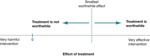
Figure 4.3 Tree plot of effect size. Reproduced with permission from Herbert et al, Practice Evidence-Based Physiotherapy, 2nd ed, Elsevier, 2011.16
In the situation where the entire confidence interval is below the smallest clinically worthwhile effect, this is a useful result. It is useful because at least we know with some certainty that the intervention is not likely to produce a clinically worthwhile effect. Similarly, when an entire confidence interval is above the smallest clinically worthwhile effect, this is a clear result, as we know with some certainty that the intervention is likely to produce a clinically worthwhile effect.
However, in the knee osteoarthritis trial, we calculated the 95% confidence interval to be 0.05 cm to 1.27 cm. The lower value is below 0.8 cm (20% of the initial pain level that we nominated as the smallest clinically worthwhile effect), but the upper value is above 0.8 cm. We can see this clearly if we mark the confidence interval onto a tree plot (see Figure 4.4, tree plot A). This indicates that there is uncertainty about whether there is a clinically worthwhile effect occurring or not.
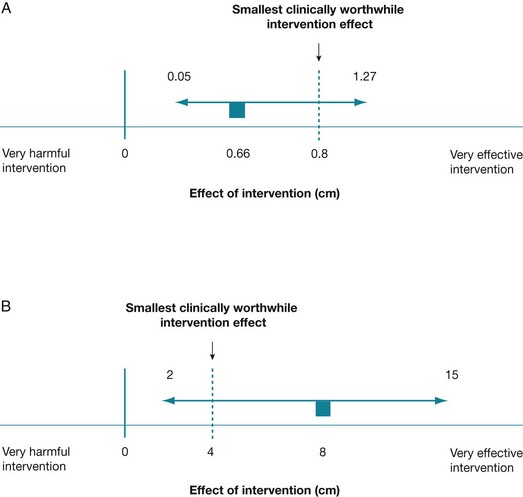
Figure 4.4 Tree plots showing the effect size, the smallest clinically worthwhile effect and the confidence interval associated with the effect size.
In tree plot A, the estimate of the intervention effect size (0.66 cm) sits below the smallest clinically worthwhile effect of 0.8 cm and the confidence interval (0.05 cm to 1.27 cm) spans the smallest clinically worthwhile effect of 0.8 cm. The estimate of the intervention effect size is indicated as a small square, the 95% confidence interval about this estimate is shown as a horizontal line and the dotted line indicates the supposed smallest clinically worthwhile intervention effect.
In tree plot B, the estimate of the intervention effect size (8) is above the smallest clinically worthwhile effect (4) and the confidence interval (2 to 15) spans the smallest clinically worthwhile effect.
When the confidence interval spans the smallest clinically worthwhile effect, it is more difficult to interpret clinical significance. In this situation, the true effect of the intervention could lie either above the smallest clinically worthwhile effect or below it. In other words, there is a chance that the intervention may produce a clinically worthwhile effect, but there is also a chance that it may not. Another example of this is illustrated in tree plot B in Figure 4.4, using the data from a randomised controlled trial that investigated the efficacy of a guided self-management program for people with asthma compared with traditional asthma treatment.28 One of the main outcome measures in this study was quality of life, which was measured using a section of the St George Respiratory Questionnaire. The total score for this outcome measure can range from –50 to +50, with positive scores indicating improvement and negative scores indicating deterioration in quality of life compared with one year ago. At the 12-month follow-up, the difference between the means of the two groups (that is, the intervention effect size) was 8 points (in favour of the self-management group), with a 95% confidence interval of 2 to 15. This difference was statistically significant (p = 0.009). Let us assume that we nominate a difference of 4 points to be the smallest clinically worthwhile effect for this example. In this example, the mean difference (8) is above what we have chosen as the smallest clinically worthwhile effect (4), but the confidence interval includes some values that are above the worthwhile effect and some values that are below it. If the true intervention effect was at the upper limit of the confidence interval (at 15), we would consider the intervention to be worthwhile, while if the true intervention effect was at the lower limit of the confidence interval (2), we may not. So, although we would probably conclude that the effect of this self-management intervention on quality of life was clinically significant, this conclusion would be made with a degree of uncertainty.
The situation of a confidence interval spanning the smallest clinically worthwhile effect is a common one, and there are two main reasons why it can occur. First, it can occur when a study has a small sample size and therefore low power. The concept of power was explained in Chapter 2. As we also saw in Chapter 2, the smaller the sample size of a study, the wider (that is, less precise) the confidence interval is, which makes it more likely that the confidence interval will span the worthwhile effect. Second, it can occur because many interventions only have fairly small intervention effects, meaning that their true effects are close to the smallest clinically worthwhile effect. As a consequence, they need to have very narrow confidence intervals if the confidence interval is going to avoid spanning the smallest worthwhile effect.16 As we just discussed, this typically means that a very large sample size is needed. In allied health studies in particular, this can be difficult to achieve.
There are two ways that you, as a health professional who is trying to decide whether to use an intervention with a patient, can deal with this uncertainty:16
• Accept the uncertainty and make your decision according to whether the difference between the group means is higher or lower than the smallest clinically worthwhile effect. However, keep the confidence interval in mind as it indicates the degree of doubt that you should have about this estimate.
• Try to increase the certainty by searching for similar studies and establishing whether the findings are replicated in other studies. This is one of the advantages of a systematic review, in particular a meta-analysis, as combining the results from multiple trials increases the sample size. The consequence of this is usually a more narrow (more precise) confidence interval which is less likely to span the smallest clinically worthwhile effect. Systematic reviews and meta-analyses are discussed in detail in Chapter 12.
Dichotomous outcomes—size of the treatment effect
Often the outcomes that are reported in a trial will be presented as dichotomous data. As we saw at the beginning of this results section, these are data for which there are only two possible values. It is worth being aware that data measured using a continuous scale can also be categorised, using a certain cut-off point on the scale, so that the data become dichotomised. For example, data on a 10-point visual analogue pain scale can be arbitrarily dichotomised around a cut-off point of 3 (or any point that the researchers choose), so that a pain score of 3 or less is categorised as mild pain and a score of above 3 is categorised as moderate/severe pain. By doing this, the researchers have converted continuous data into data that can be analysed as dichotomous data.
Health professionals and patients are often interested in comparative results—the outcome in one group relative to the outcome in the other group. This overall (comparative) consideration is one of risk. Before getting into the details, let us briefly review the concept of risk. Risk is simply the chance, or probability, of an event occurring. A probability can be described by numbers, ranging from 0 to 1, and is a proportion or ratio. Risks and probabilities are usually expressed as a decimal, such as 0.1667, which is the same as 16.67%. Risk can be expressed in various ways (but using the same data).29 We will consider each of these in turn:
1. relative risk (or the flip side of this, which is referred to as relative benefit)
2. relative risk reduction (or relative benefit increase)
Risk and relative risk (or relative benefit)
Consider a hypothetical study that investigated the use of relaxation training to prevent the recurrence of migraines. The control group (n = 100) received no intervention and is compared with the intervention group (n = 100) who received the relaxation training. Suppose that at the end of the 1-month trial, 25 of the participants in the control group had had a migraine.
• The risk for recurrence of migraine in the control group can be calculated as 25/100, which can be expressed as 25%, or a risk of recurrence of 0.25. This is also known as the Control Event Rate (CER).
• If, in the relaxation group, only 5 participants had had a migraine, the risk of recurrence would be 5% (5/100) or 0.05. This is sometimes referred to as the experimental event rate (EER).
These data can be represented graphically, as in Figure 4.5.
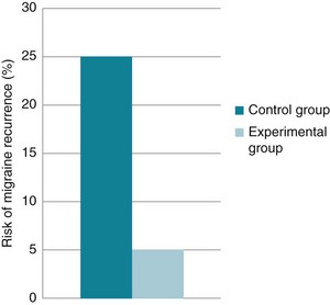
Figure 4.5 Risk of migraine recurrence in the control group and intervention group in a hypothetical study.
We are interested in the comparison between groups. One way of doing this is to consider the relative risk—a ratio of the probability of the event occurring in the intervention group versus in the control group.30 In other words, relative risk is the risk or probability of the event in the intervention group divided by that in the control group. The term relative risk is being increasingly replaced by use of the term risk ratio—this describes the same concept, but the term reflects that it is a ratio that is being referred to. In the migraine study, the relative risk (that is, the risk ratio) would be calculated by dividing the experimental event rate (EER) by the control event rate (CER):

This can be expressed as: ‘the risk of having a recurrence of migraine for those in the relaxation group is 20% of the risk in the control group’.
You may remember that when we were discussing continuous outcomes, the no effect value was zero (when referring to the difference between group means). When referring to relative risk, the no effect value (the value that indicates that there is no difference between groups) is 1. This is because if the risk is the same in both groups (for example, 0.25 in one group and 0.25 in the other group), there would be no difference and the relative risk (risk ratio) would be 0.25/0.25 = 1. Therefore, a relative risk (risk ratio) of less than 1 indicates lower risk—that is, a benefit from the intervention.30
If we are evaluating a study that aimed to improve an outcome (that is, make it more likely to occur) rather than reducing a risk, we might instead consider using the equivalent concept of relative benefit. For example, in a study that evaluated the effectiveness of phonological training to increase reading accuracy among children with learning disabilities, we could calculate relative benefit as the study was about improving an outcome, not reducing the risk of it happening.
Sometimes a study will report an odds ratio instead of relative risk. It is similar, except that an odds ratio refers to a ratio of odds, rather than a ratio of risks. The odds ratio is the ratio of the odds of an event for those in the intervention group compared with the odds of an event in the control group. Odds are derived by dividing the event rate by the non-event rate for each group. The odds ratio is calculated by the following formula, where CER is the ‘control event rate’ and EER refers to the ‘experimental event rate’:

Also, some studies may report the intervention effect as a hazard ratio. This typically occurs when a survival analysis has been performed. A hazard ratio is broadly similar in concept to a risk ratio (relative risk) and so can be interpreted in a similar manner—that is, it describes how many times more (or less) likely a participant is to experience the event at a particular point in time if they were in the intervention group rather than the control group.
Relative risk reduction (or relative benefit increase)
Relative risk reduction is another way of expressing the difference between the two groups, and is simply the proportional reduction in an event of interest (for example, falls) in the intervention group compared with the control group, at a specified time point. Again, there is a flip side of this concept, which is known as relative benefit increase. When appraising an article and using this concept, you need to keep in mind whether you are considering negative or positive outcomes:
• Relative risk reduction (RRR) is used for expressing the reduction in risk of a negative outcome (such as falling).
• Relative benefit increase (RBI) is used for expressing an increase in the probability of a beneficial outcome (such as returning to work).
The formula that can be used for calculating relative risk reduction or relative benefit increase is:

Remember, we have said that the CER is the ‘control event rate’ and EER refers to the ‘experimental event rate’.29 The CER is simply the proportion of participants in the control group who experienced the event of interest. In our study of relaxation training to reduce migraines, this was 25% (or 0.25). Similarly, the EER is the proportion of participants in the intervention (experimental) group who experienced the event of interest. This was 5% (or 0.05) in the relaxation study.
Using our relaxation training study as an illustration, relative risk reduction can be calculated as: (0.25 – 0.05) ÷ 0.25 = 0.80. We could multiply this by 100 to get 80% and report that the relaxation training reduced the rate of migraines by 80%.
Alternatively, if you already know the relative risk, then the relative risk reduction can be calculated easily using the formula:

In our example, where the relative risk (RR) is 0.20, the relative risk reduction is 0.80 or 80% (calculated as 1 – 0.20).
The main difficulty in the use of relative risk reduction is that it does not reflect the baseline risk of the event.31 This means that as a reader you are unable to discriminate between small intervention effects and large ones. Baseline risk has an important role to play. To understand this, you need to think about the risk in different populations. For example, in the general population the risk of migraine might be around 5–10% (depending on factors such as gender, age, and so on). Reducing the risk of migraine in a population that has a low risk to start with is very hard to achieve, and any risk reduction that is found would be fairly small (and as you will see in the next section, absolute risk reduction would be smaller still). However, in a population of people who commonly have migraines, the risk of recurrence is much higher and it would, therefore, be easier to achieve a larger relative risk reduction. Interventions that reduce the risk in populations who are at high risk of the event under consideration are likely to be clinically worthwhile.32
Another difficulty with the use of the relative risk reduction concept is that it can make results seem more impressive than they really are. Expressing the effects of an intervention in relative terms will result in larger percentages than when the same intervention is expressed in absolute terms. For example, suppose the use of a particular type of mattress reduced the risk of pressure sores from 0.05 to 0.025. In relative terms, the mattress reduces the risk by 50% (calculated by: 0.025 ÷ 0.05 = 0.5 or 50%), while in absolute terms it reduces the risk by 2.5% (calculated by: 0.05 – 0.025 = 0.025 or 2.5%). Similarly, in the hypothetical trial on relaxation training for reducing recurrence of migraines the relative risk reduction seems an impressive 80% but, as we will see later, the absolute difference in the rate of events between groups is only 20%. So we can see that the concept of relative risk reduction can inflate the appearance of intervention effectiveness.
You should also be aware that two studies might have the same relative risk reduction but there may be a large difference in the absolute risk reduction. As we saw in the example above about reducing the risk of pressure sores by using a particular type of mattress, a reduction in risk from 0.05 to 0.025 reduces the relative risk by 50%, while in absolute terms it reduces the risk by 2.5%. Let us say that another study found that the risk of pressure sores in a very-high-risk group of people was reduced from 0.8 to 0.4 because of the intervention (the mattress). In relative terms, although the mattress reduced the relative risk by 50% (calculated by: 0.8 ÷ 0.4 = 0.5 or 50%), the absolute risk reduction is 40%, which is a more clinically valuable result than the absolute risk reduction of 2.5% that the first study found.
Absolute risk reduction (or absolute benefit increase)
Another way of presenting information about dichotomous outcomes is by referring to the absolute risk reduction. The absolute risk reduction is simply the absolute arithmetic difference in event rates between the experimental (intervention) and the control groups.33 This is shown graphically in Figure 4.6. Absolute values are simply the value of a number, regardless of its sign (positive or negative sign). The notation used for absolute values is vertical bars either side of the value, for example: |x|. The absolute arithmetic difference for risk reduction is calculated as: |EER – CER|. As with the previous methods of calculating risk that we have explained, there is a flip side to this concept. This is known as absolute benefit increase and is used when referring to a beneficial outcome (such as being discharged home instead of discharged to residential care).
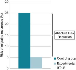
Figure 4.6 Absolute risk reduction for migraine recurrence in a hypothetical study of relaxation training.
In our hypothetical relaxation study for reducing recurrence of migraine, the absolute risk reduction would be 25% – 5% = 20%. This could be expressed as: ‘the absolute risk of having a migraine recurrence was 20% less in the people who were in the relaxation group compared with those in the control group’.
A big absolute risk reduction indicates that the intervention is very effective, but how big is big enough to be considered clinically significant? A more meaningful measure, known as number needed to treat, can be used instead.
Number needed to treat
We saw that the absolute risk reduction of having migraine recurrence in the relaxation study was calculated as 20%, but is this clinically worthwhile? Number needed to treat (NNT) is a method of making the magnitude of the absolute risk reduction more explicit and is a more clinically useful concept.30 The number needed to treat is simply the inverse of absolute risk reduction,34 and is calculated as:
It tells you the number of people who would need to be treated to achieve the event of interest once. In the trial of relaxation training for preventing migraine recurrence, the number needed to treat is 1 ÷ (0.25 – 0.05) = 5. So, in this example, you would have to treat 5 people for 1 month with the hypothetical relaxation intervention to prevent one (extra) person from having a recurrence of migraine (when compared with the control group). Obviously, a smaller number needed to treat is better than a large one. An intervention that has a smaller number needed to treat is more effective than an intervention that has a larger number needed to treat.
This concept of number needed to treat makes it easier to consider clinical significance, as you can more easily weigh up the benefits of preventing the event in one person against the costs and risks of providing the intervention. The size of the smallest clinically worthwhile effect (that is, the smallest worthwhile number needed to treat) will then depend on the seriousness of the event and the costs and risks of the intervention.
Another handy feature when using number needed to treat is that you can compare two different interventions (that are trying to achieve the same outcome) that have the same number needed to treat but have other features that are different. For example, one of the interventions may have a shorter intervention time and/or result in fewer side effects and/or be more convenient to patients and/or be less expensive. It is important to consider features such as these that a particular intervention has when making a decision about which intervention to use with a patient.
Applying results to your clinical situation
Most health professionals find it difficult to translate the results from studies to individual patients or to specific clinical situations, as studies usually only tell us about the average effects of the intervention. Further, the participants who took part in the study may be different to the patients that we see, and the intervention may differ to the intervention that we use. However, as a rough guide, if your patient is ‘healthier’ or the situation that you are considering is more optimistic than that in the study, the number needed to treat would be lower, the relative benefit increase would be higher, the mean difference would be larger, and so on. If, however, your patient is ‘worse off’ or the situation that you are considering is worse than that in the study, the number needed to treat would be higher, the relative benefit increase would be lower, the mean difference would be smaller, and so on. A solution to applying the results of a trial to patients with higher or lower levels of risk has been described by Straus and Sackett35 and you may wish to read their article to learn more about this.
Dichotomous outcomes—precision of the treatment effect
Confidence intervals are also important to consider when examining dichotomous outcomes as, again, they indicate how much uncertainty is associated with the estimate of the intervention effect (in other words, the precision or accuracy of the estimate). The principles of confidence intervals associated with dichotomous data are similar to those for continuous data, but there is one very important difference to consider—what is the appropriate no effect value to use?
• For effect size estimates where subtraction is involved, such as mean differences (for continuous outcomes) and absolute risk reductions, the no effect value is 0.
• For effect sizes that involve division, such as risk ratios and odds ratios, the no effect value is 1.
Therefore, you can see that it is important to consider the type of effect measure you are interpreting in order to reliably interpret the confidence interval. The same general principle applies, though—a 95% confidence interval that does not include the no effect value indicates that the result is statistically significant. Table 4.1 presents a summary of the dichotomous effect measures, including what the no effect value is, that have been discussed in this section of the chapter.
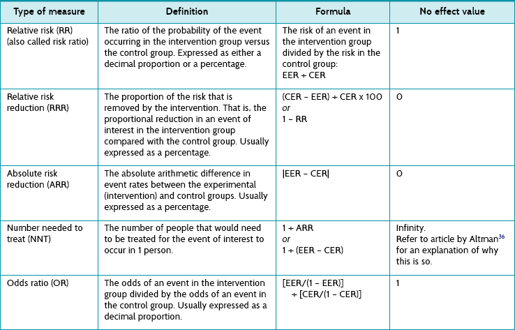
As we could do with continuous outcomes, if the confidence interval has not been provided by the authors of the article it can be possible to calculate an approximate confidence interval. This is illustrated in Box 4.3. Again, a simplified version of the more complex equation is used, but the confidence interval that is calculated is sufficient for use by health professionals who wish to use the information to assist in clinical decision making. Once you know the confidence interval for the absolute risk reduction, if you wish you could plot it, the effect estimate and the smallest clinically worthwhile effect on a tree plot in the same way that we did for continuous outcomes in Figure 4.4.
Box 4.3 How to calculate the confidence interval (CI) for absolute risk reduction
A formula32 that can be used is:

where nav = average of the group sizes.
For our study of relaxation training, the 95% confidence interval for the absolute risk reduction would be:


This tells us that the best estimate of the absolute risk reduction achieved from the relaxation training is 35% and that the 95% confidence interval extends from 15% to 35%.
Calculating the confidence intervals for number needed to treat is fairly straightforward, as you just use the inverse of the numbers in the confidence interval of the absolute risk reduction.30 However, understanding how to interpret the confidence intervals for number needed to treat can be complicated, and the article by Altman36 is recommended to understand this in detail.
When making sense of the results of a randomised controlled trial, one further issue that you should be aware of is that trials usually report results from many different outcomes. With so much information to process it may be helpful, in some cases, for you to focus your attention on the main outcome(s) of the trial, the outcome(s) of interest to the question that you initially formed and/or the outcome that is of interest to your patient. If you have got to this point and determined that the article that you have been appraising not only appears to be reasonably free of bias but also contains some clinically important results, you then proceed to look at whether you can apply the results from the study to your patient or clinical situation. This is the third and final step of the critical appraisal process that we described in Chapter 1.
How can we use this evidence to inform practice?
If you have decided that the validity of the study you are appraising is adequate and that the results are clinically important, the final step of the critical appraisal process is to consider the application of this information to the clinical situation that prompted your original clinical question. To do this, there are a few important questions which should be considered:
• Do the results apply to your patient or situation?
• Do the benefits found outweigh any harm, costs and/or inconveniences that are involved with the intervention?
• What other factors might need to be considered when applying this evidence?
Do the results apply to your patient or situation?
When considering whether the results apply to your patient or situation, you essentially need to assess whether your patient is so different from the participants in the study that you cannot apply the results of the study that you have been reading to your patient or situation. So, rather than just thinking about the study's eligibility criteria with respect to your patient, are the differences problematic enough that the results should not be applied? Further to this, results can sometimes be individualised to a particular patient by considering the individual benefit and harm for that patient. There is some complexity involved in doing so, which is beyond the scope of this book. If you wish to learn about this further, you are advised to read the article by Glasziou and Irwig39 to understand how this may be done.
Do the benefits found outweigh any harm, costs and/or inconveniences that are involved with the intervention?
Understanding whether benefits outweigh harms or costs requires using information about benefits that is given in terms of the size of the intervention effect (e.g. mean differences, relative risk reduction, number needed to treat) and comparing this against possible harms or even inconveniences. When information about harm and cost is provided in the article, this is relatively straightforward. However, this type of information is often not provided and some estimate of the costs associated with the intervention might need to be made. Information about harm is obviously more difficult to estimate, and other sources might need to be consulted to get a sense of the potential harms involved. This is a grey area of practice in which clinical experience and discussion with patients about their preferences and values become very important.
What other factors might need to be considered when applying this evidence?
A further important question to consider is: what other factors might need to be considered when applying this evidence? When you are thinking about what other factors affect the delivery of an intervention, there are a few key questions that you can ask, such as:
• How many sessions might be involved or how long would the patient need to stay in hospital?
• How far would the patient (or the health professional) need to travel?
• Are the resources (for example, any equipment that is needed) available to deliver the intervention?
• Do you or other health professionals working with you have the skills to provide the intervention?
A central component of applying research evidence to your patient is discussing the information with them. The success of many interventions is dependent on the health professional successfully providing the patient with appropriate information.
Involving the patient in the decision-making process is important, and this is discussed further in Chapter 14. In Chapter 1 we emphasised the need for integrating information from patients, clinical experience, research and the practice context. To do so is the art of evidence-based practice. Integrating so many pieces of information from many different sources is certainly an art form and one that requires clinical reasoning and judgment. The roles of clinical reasoning and judgment are discussed further in Chapter 15.
References
1. Portney, L, Watkins, M. Foundations of clinical research: applications to practice. Upper Saddle River, NJ: Prentice Hall Health; 2000.
2. Deeks, J, Dinnes, J, D'Amico, R, et al. Evaluating non-randomised intervention studies. Health Technol Assess. 2003; 7:1–186.
3. Allan, L, Hays, H, Jensen, N, et al. Randomised crossover trial of transdermal fentanyl and sustained release oral morphine for treating chronic non-cancer pain. BMJ. 2001; 322:1154–1158.
4. Clemson, L, Cumming, R, Kendig, H, et al. The effectiveness of a community-based program for reducing the incidence of falls in the elderly: a randomised trial. J Am Geriatr Soc. 2004; 52:1487–1494.
5. Guyatt, GH, Sackett, DL, Cook, DJ. Users’ guides to the medical literature. II. How to use an article about therapy or prevention. JAMA. 1993; 270:2598–2601.
6. Maher, C, Sherrington, C, Herbert, R, et al. Reliability of the PEDro scale for rating quality of randomised controlled trials. Phys Ther. 2003; 83:713–721.
7. Shulz, K, Chalmers, I, Hayes, R, et al. Empirical evidence of bias: dimensions of methodological quality associated with estimates of treatment effects in controlled trials. JAMA. 1995; 273:408–412.
8. Kunz, R, Vist, G, Oxman, A. Randomisation to protect against selection bias in healthcare trials. Cochrane Database Syst Rev. (2):2007. [MR000012. doi: 10.1002/14651858.MR000012.pub2].
9. Altman, DG, Bland, JM. Treatment allocation in controlled trials: why randomise? BMJ. 1999; 318:1209.
10. Hewitt, C, Torgerson, D. Is restricted randomisation necessary? BMJ. 2006; 332:1506–1508.
11. El-Mohandes, A, Katz, K, El-Khorazaty, M, et al. The effect of a parenting education program on the use of preventive paediatric health care services among low-income, minority mothers: a randomised, controlled study. Pediatrics. 2003; 111:1324–1332.
12. Altman, D, Schulz, K, Moher, D, et al. The revised CONSORT statement for reporting randomised trials: explanation and elaboration. Ann Intern Med. 2001; 134:663–694.
13. Pildal, J, Chan, AW, Hróbjartsson, A, et al. Comparison of descriptions of allocation concealment in trial protocols and the published reports: cohort study. BMJ. 2005; 330:1049–1054.
14. Bennett, S, McKenna, K, McCluskey, A, et al. Evidence for occupational therapy interventions: status of effectiveness research indexed in the OTseeker database. Br J Occup Ther. 2007; 70:426–430.
15. Roberts, C, Torgerson, D. Understanding controlled trials: baseline imbalance in randomised controlled trials. BMJ. 1999; 319:185.
16. Herbert, R, Jamtvedt, G, Hagen, K, et al. Practical evidence-based physiotherapy, 2nd ed. Edinburgh: Elsevier; 2011.
17. Dumville, J, Torgerson, D, Hewitt, CE. Reporting attrition in randomised controlled trials. BMJ. 2006; 332:969–971.
18. Schulz, K, Altman, D, Moher, D, the CONSORT Group. CONSORT 2010 statement: updated guidelines for reporting parallel-group randomised trials. BMJ. 340, 2010. [doi: 10.1136/bmj.c332].
19. Higgins, J, Altman, D, Sterne, J, Chapter 8: Assessing risk of bias in included studiesHiggins J, Green S, eds. Cochrane Handbook for Systematic Reviews of Interventions. Version 5.1.0 (updated March 2011). The Cochrane Collaboration: 2011. Online Available www.cochrane-handbook.org
20. Hollis, S, Campbell, F. What is meant by intention to treat analysis? Survey of published randomised controlled trials. BMJ. 1999; 319:670–674.
21. Ottenbacher, K, Maas, F. How to detect effects: statistical power and evidence-based practice in occupational therapy research. Am J Occup Ther. 1999; 53:181–188.
22. Heuts, P, de Bie, R, Drietelaar, M, et al. Self-management in osteoarthritis of hip or knee: a randomised clinical trial in a primary healthcare setting. J Rheumatol. 2005; 32:543–549.
23. Cohen, J. Statistical power analysis for the behavioural sciences, 2nd ed. Hillsdale, NJ: Lawrence Erlbaum; 1988.
24. Norman, G, Sloan, J, Wyrwich, K. Interpretation of changes in health-related quality of life: the remarkable universality of half a standard deviation. Med Care. 2003; 41:582–592.
25. Guyatt, G. Making sense of quality-of-life data. Med Care. 2000; 39(II):175–179.
26. Herbert, R. How to estimate treatment effects from reports of clinical trials. I: continuous outcomes. Aust J Physiother. 2000; 46:229–235.
27. Altman, D, Bland, J. Absence of evidence is not evidence of absence. BMJ. 1995; 311:485.
28. Lahdensuo, A, Haahtela, T, Herrala, J, et al. Randomised comparison of guided self-management and traditional treatment of asthma over one year. BMJ. 1996; 312:748–752.
29. Guyatt, G, Sackett, D, Cook, D. Users' guide to the medical literature: II. How to use an article about therapy or prevention: B. what were the results and will they help me in caring for my patients? JAMA. 1994; 271:59–63.
30. Cook, R, Sackett, D. The number needed to treat: a clinically useful measure of treatment effect. BMJ. 1995; 310:452–454.
31. Sackett, D, Richardson, W, Rosenberg, W, et al. Evidence-based medicine. How to practice and teach EBM. New York: Churchill Livingstone; 1997.
32. Herbert, R. How to estimate treatment effects from reports of clinical trials. II: Dichotomous outcomes. Aust J Physiother. 2000; 46:309–313.
33. Centre for Evidence-Based Medicine, Glossary. University of Oxford, Oxford, 31 May 2012. Online Available www.cebm.net/index.aspx?o=1116
34. Laupacis, A, Sackett, D, Roberts, R. An assessment of clinically useful measures of the consequences of treatment. N Engl J Med. 1988; 318:1728–1733.
35. Straus, S, Sackett, D. Applying evidence to the individual patient. Ann Oncol. 1999; 10:29–32.
36. Altman, D. Confidence intervals for the number needed to treat. BMJ. 1998; 317:1309–1312.
37. Cumming, R. Intervention strategies and risk-factor modification for falls prevention: a review of recent intervention studies. Clin Geriatr Med. 2002; 18:175–189.
38. Campbell, A, Robertson, M, Gardner, M, et al. Falls prevention over 2 years: a randomised controlled trial in women 80 years and older. Age Ageing. 1999; 28:513–518.
39. Glasziou, P, Irwig, L. An evidence based approach to individualising treatment. BMJ. 1995; 311:1356–1359.