CHAPTER 17
Emile L. Boulpaep
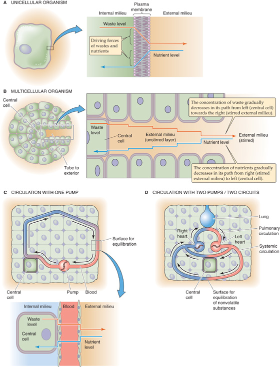
Isolated single cells and small organisms do not have a circulatory system. They can meet their metabolic needs by the simple processes of diffusion and convection of solutes from the external to the internal milieu (Fig. 17-1A). The requirement for a circulatory system is an evolutionary consequence of the increasing size and complexity of multicellular organisms. Simple diffusion (see Chapter 5) is not adequate to supply nutrients to centrally located cells or to eliminate waste products; in large organisms, the distances separating the central cells from the external milieu are too long. A simple closed-end tube (Fig. 17-1B), penetrating from the extracellular compartment and feeding a central cell deep in the core of the organism, would not be sufficient. The concentration of nutrients inside the tube would become very low at its closed end because of both the uptake of these nutrients by the cell and the long path for re-supply leading to the cell. Conversely, the concentration of waste products inside the tube would become very high at the closed end. Such a tube represents a long unstirred layer; as a result, the concentration gradients for both nutrients and wastes across the membrane of the central cell are very small.
Figure 17-1 Role of the circulatory system in promoting diffusion. In C, nutrients and wastes exchange across two barriers: a surface for equilibration between the external milieu and blood, and another surface between blood and the central cell. Inset, Blood is the conduit that connects the external milieu (e.g., lumina of lung, gut, and kidney) to the internal milieu (i.e., extracellular fluid bathing central cells). In D, the system is far more efficient, using one circuit for exchange of gases with the external milieu and another circuit for exchange of nutrients and nongaseous wastes.
In complex organisms, a circulatory system provides a steep concentration gradient from the blood to the central cells for nutrients and in the opposite direction for waste products. Maintenance of such steep intracellular-to-extracellular concentration gradients requires a fast convection system that rapidly circulates fluid between surfaces that equilibrate with the external milieu (e.g., the lung, gut, and kidney epithelia) and individual central cells deep inside the organism (Fig. 17-1C). In mammals and birds, the exchange of gases with the external milieu is so important that they have evolved a two-pump, dual circulatory system (Fig. 17-1D) that delivers the full output of the “heart” to the lungs (see Chapter 31).
The primary role of the circulatory system is the distribution of dissolved gases and other molecules for nutrition, growth, and repair. Secondary roles have also evolved: (1) fast chemical signaling to cells by means of circulating hormones or neurotransmitters, (2) dissipation of heat by delivery of heat from the core to the surface of the body, and (3) mediation of inflammatory and host defense responses against invading microorganisms.
The circulatory system of humans integrates three basic functional parts, or organs: a pump (the heart) that circulates a liquid (the blood) through a set of containers (the vessels). This integrated system is able to adapt to the changing circumstances of normal life. Demand on the circulation fluctuates widely between sleep and wakefulness, between rest and exercise, with acceleration/deceleration, during changes in body position or intrathoracic pressure, during digestion, and under emotional or thermal stress. To meet these variable demands, the entire system requires sophisticated and integrated regulation.
A remarkable pump, weighing ~300 g, drives the human circulation. The heart really consists of two pumps, the left-sided heart, or main pump, and the right-sided heart, or boost pump (Fig. 17-1D). These operate in series and require a delicate equalization of their outputs. The output of each pump is ~5 L/min, but this can easily increase 5-fold during exercise.
During a 75-year lifetime, the two ventricles combined pump 400 million liters of blood (enough to fill a lake 1 km long, 40 m wide, and 10 m deep). The circulating fluid itself is an organ, kept in a liquid state by mechanisms that actively prevent cell-cell adhesion and coagulation. With each heartbeat, the ventricles impart the energy necessary to circulate the blood by generating the pressure head that drives the flow of blood through the vascular system. On the basis of its anatomy, we can divide this system of tubes into two main circuits: the systemic and the pulmonary circulations (Fig. 17-1D). We could also divide the vascular system into a high-pressure part (extending from the contracting left ventricle to the systemic capillaries) and a low-pressure part (extending from the systemic capillaries, through the right side of the heart, across the pulmonary circulation and left atrium, and into the left ventricle in its relaxed state). The vessels also respond to the changing metabolic demands of the tissues they supply by directing blood flow to (or away from) tissues as demands change. The circulatory system is also self-repairing/self-expanding. Endothelial cells lining vessels mend the surfaces of existing blood vessels and generate new vessels (angiogenesis).
Some of the most important life-threatening human diseases are caused by failure of the heart as a pump (e.g., congestive heart failure), failure of the blood as an effective liquid organ (e.g., thrombosis and embolism), or failure of the vasculature either as a competent container (e.g., hemorrhage) or as an efficient distribution system (e.g., atherosclerosis). Moreover, failure of the normal interactions among these three organs can by itself elicit or aggravate many human pathological processes.
To keep concepts simple, first think of the left side of the heart as a constant pressure generator that maintains a steady mean arterial pressure at its exit (i.e., the aorta). In other words, assume that blood flow throughout the circulation is steady or nonpulsatile (later in the chapter, see discussion of the consequences of normal cyclic variations in flow and pressure that occur as the result of the heartbeat). As a further simplification, assume that the entire systemic circulation is a single, straight tube.
To understand the steady flow of blood, driven by a constant pressure head, we can apply classical hydrodynamic laws. The most important law is analogous to Ohm’s law of electricity:
That is, the pressure difference (ΔP) between an upstream point (pressure P1) and a downstream site (pressure P2) is equal to the product of the flow (F) and the resistance (R) between those two points (Fig. 17-2). Ohm’s law of hydrodynamics holds at any instant in time, regardless of how simple or how complicated the circuit. This equation also does not require any assumptions about whether the vessels are rigid or compliant, as long as R is constant.
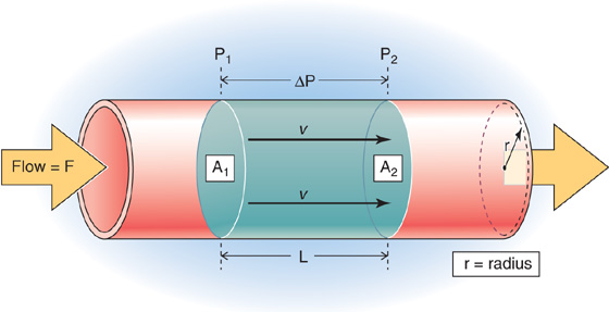
Figure 17-2 Flow through a straight tube. The flow (F) between a high-pressure point (P1) and a low-pressure point (P2) is proportional to pressure difference (ΔP). A1 and A2 are cross-sectional areas at these two points. A cylindrical bolus of fluid—between the disks at points 1 and 2—moves down the tube with a linear velocity v.
In reality, the pressure difference (ΔP) between the beginning and end points of the human systemic circulation—that is, between the high-pressure side (aorta) and the low-pressure side (vena cava)—turns out to be fairly constant over time. Thus, the heart behaves more like a generator of a constant pressure head than a generator of constant flow, at least within physiological limits. Indeed, flow (F), the output of the left side of the heart, is quite variable in time and depends greatly on the physiological circumstances (e.g., whether one is active or at rest). Like flow, resistance (R) varies with time; in addition, it varies with location within the body. The overall resistance of the circulation reflects the contributions of a complex network of vessels in both the systemic and pulmonary circuits.
Blood can take many different pathways from the left side of the heart to the right side of the heart (Fig. 17-3): (1) a single capillary bed (e.g., coronary capillaries), (2) two capillary beds in series (e.g., glomerular and peritubular capillaries in the kidney), or (3) two capillary beds in parallel that subsequently merge and feed into a single capillary bed in series (e.g., the parallel splenic and mesenteric circulations, which merge on entering the portal hepatic circulation). In contrast, blood flow from the right side of the heart to the left side of the heart can take only a single pathway, across a single capillary bed in the pulmonary circulation. Finally, some blood also courses from the left side of the heart directly back to the left side of the heart across shunt pathways, the most important of which is the bronchial circulation.
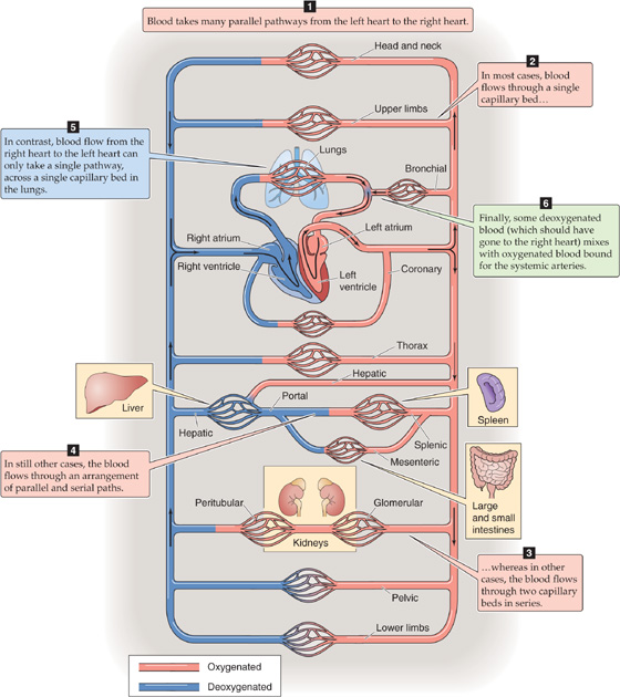
Figure 17-3 Circulatory beds.
The overall resistance (Rtotal) across a circulatory bed results from parallel and serial arrangements of branches and is governed by laws similar to those for the electrical resistance of DC circuits. For multiple resistance elements (R1, R2, R3, …) arranged in series:

For multiple elements arranged in parallel:
Physicists measure pressure in the units of pascals, g/cm2, or dynes/cm2. However, physiologists most often gauge blood pressure by the height it can drive a column of liquid. This pressure is

where ρ is the density of the liquid in the column, g is the gravitational constant, and h is the height of the column. Therefore, if we neglect variations in g and know ρ for the fluid in the column (usually water or mercury), we can take the height of the liquid column as a measure of blood pressure. Physiologists usually express this pressure in millimeters of mercury (mm Hg) or centimeters of water (cm H2O). Clinicians use the classical blood pressure gauge (sphygmomanometer) to report arterial blood pressure in millimeters of mercury.
Pressure is never expressed in absolute terms but as a pressure difference ΔP relative to some “reference” pressure. We can make this concept intuitively clear by considering pressure as a force F applied to a surface area A.

If we apply a force to one side of a free-swinging door, we cannot predict the direction the door will move unless we know what force a colleague may be applying on the opposite side. In other words, we can define a movement or distortion of a mechanical system only by the difference between two forces. In electricity, we compare the difference between two voltages. In hemodynamics, we compare the difference between two pressures. When it is not explicitly stated, the reference pressure in human physiology is the atmospheric or barometric pressure (PB). Because PB on earth is never zero, a pressure reading obtained at some site within the circulation, and referred to PB, actually does not express the absolute pressure in that blood vessel but rather the difference between the pressure inside the vessel and PB.
Because a pressure difference is always between two points—and these two points are separated by some distance (Δx) and have a spatial orientation to one another—we can define a pressure gradient (ΔP/Δx) with a spatial orientation. Considering orientation, we can define three different kinds of pressure differences in the circulation:
1. Driving pressure. In Figure 17-4, the ΔP between points x1 and x2 inside the vessel—along the axis of the vessel—is the axial pressure difference. Because this ΔP causes blood to flow from x1 to x2, it is also known as the driving pressure. In the circulation, the driving pressure is the ΔP between the arterial and venous ends of the systemic (or pulmonary) circulation, and it governs blood flow. Indeed, this is the only ΔP we need to consider to understand flow in horizontal rigid tubes (Fig. 17-2).
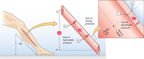
Figure 17-4 Three kinds of pressure differences, and their axes, in a blood vessel.
2. Transmural pressure. The ΔP in Figure 17-4 between point r1 (inside the vessel) and r2 (just outside the vessel)—along the radial axis—is an example of a radial pressure difference. Although there is normally no pressure difference through the blood along the radial axis, the pressure drops steeply across the vessel wall itself. The ΔP between r1 and r2 is the transmural pressure, that is, the difference between the intravascular pressure and the tissue pressure. Because blood vessels are distensible, transmural pressure governs vessel diameter, which is in turn the major determinant of resistance.
3. Hydrostatic pressure. Because of the density of blood and gravitational forces, a third pressure difference arises if the vessel does not lie in a horizontal plane, as was the case in Figure 17-2. The ΔP in Figure 17-4 between point h1 (bottom of a liquid column) and h2 (top of column)—along the height axis—is the hydrostatic pressure difference P1 − P2. This ΔP is similar to the P in Equation 17-4 (here, ρ is the density of blood), and it exists even in the absence of any blood flow. If we express increasing altitude in positive units of h, then hydrostatic ΔP = −ρg(h1 − h2).
The flow of blood delivered by the heart, or the total mean flow in the circulation, is the cardiac output (CO). The output during a single heartbeat, from either the left or the right ventricle, is the stroke volume (SV). For a given heart rate (HR):

The cardiac output is usually expressed in liters per minute; at rest, it is about 5 L/min in a 70-kg human. Cardiac output depends on body size and is best normalized to body surface area. The cardiac index (L/min/m2) is the cardiac output per square meter of body surface area. The normal adult cardiac index at rest is about 3.0 L/min/m2.
The principle of continuity of flow is the principle of conservation of mass applied to flowing fluids. It requires that the volume entering the systemic or pulmonary circuit per unit time be equal to the volume leaving the circuit per unit time, assuming that no fluid has been added or subtracted in either circuit. Therefore, the flow of the right and left sides of the heart (i.e., right and left cardiac outputs) must be equal in the steady state. (See Note: Cardiac Output of the Left Heart and the Right Heart)
Flow (F) is the displacement of volume (ΔV) per unit time (Δt):
In Figure 17-2, we could be watching a bolus (the blue cylinder)—with an area A and a length L—move along the tube with a mean velocity  . During a time interval Δt, the cylinder advances by Δx, so that the volume passing some checkpoint (e.g., at P2) is (A • Δx). Thus,
This equation holds at any point along the circulation, regardless of how complicated the circulation is or how irregular the cross-sectional area.
In a physically well defined system, it is also possible to predict the flow from the geometry of the vessel and the properties of the fluid. In 1840 and 1841, Jean Poiseuille observed the flow of liquids in tubes of small diameter and derived the law associated with his name. In a straight, rigid, cylindrical tube:
This is the Poiseuille-Hagen equation, where F is the flow, ΔP is the driving pressure, r is the inner radius of the tube, l is its length, and η is the viscosity. The Poiseuille equation requires that both driving pressure and the resulting flow be constant. (See Note: The Hagen-Poiseuille Law)
Three implications of Poiseuille’s law are as follows:
1. Flow is directly proportional to the axial pressure difference, ΔP. The proportionality constant—(πr4)/(8ηl)—is the reciprocal of resistance (R), as is presented later.
2. Flow is directly proportional to the fourth power of vessel radius.
3. Flow is inversely proportional to both the length of the vessel and the viscosity of the fluid.
Unlike Ohm’s law of hydrodynamics (F = ΔP/R), which applies to all vessels, no matter how complicated, Poiseuille’s equation applies only to rigid, cylindrical tubes. Moreover, later discussion in this chapter reveals that the fluid flowing through the tube must satisfy certain conditions.
The simplest approach for expressing vascular resistance is to rearrange Ohm’s law of hydrodynamics (see Equation 17-1):
This approach is independent of geometry and is even applicable to very complex circuits, such as the entire peripheral circulation. Moreover, we can conveniently express resistance in units used by physicians for pressure (mm Hg) and flow (mL/s). Thus, the units of total peripheral resistance are mm Hg/(mL/s)—also known as peripheral resistance units (PRUs).
Alternatively, if the flow through the tube fulfills Poiseuille’s requirements, we can express “viscous” resistance in terms of the dimensions of the vessel and the viscous properties of the circulating fluid. Combining Equation 17-9 and Equation 17-10: (See Note: Viscous Resistance)
Thus, viscous resistance is proportional to the viscosity of the fluid and the length of the tube but inversely proportional to the fourth power of the radius of the blood vessel. Note that this equation makes no statement regarding the properties of the vessel wall per se. The resistance to flow results from the geometry of the fluid—as described by l and r—and the internal friction of the fluid, the viscosity (η). Viscosity is a property of the content (i.e., the fluid), unrelated to any property of the container (i.e., the vessel). (See Note: Viscous resistance)
Viscosity is an expression of the degree of slipperiness between two layers of fluid. Isaac Newton described the interaction as illustrated in Figure 17-5A. Imagine that two parallel planes of fluid, each with an area A, are moving past one another. The velocity of the first is v, and the velocity of the slightly faster moving second plane is + Δv. The difference in velocity between the moving planes is Δv, and the separation between the two planes is Δx. Thus, the velocity gradient in a direction perpendicular to the plane of shear, Δv/Δx [units: (cm/s)/cm = s−1], is the shear rate. The additional force that we must apply to the second sheet to make it move faster than the first is the shear stress. The greater the area of the sheets, the greater is the force needed to overcome the friction between them. Thus, shear stress is expressed as force per unit area (F/A). The shear stress required to produce a particular shear rate Newton defined as the viscosity:
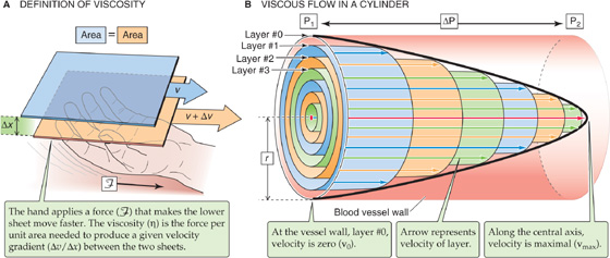
Figure 17-5 Viscosity.
Viscosity measures the resistance to sliding when layers of fluid are shearing against each other. The unit of viscosity is a poise (P). Whole blood has a viscosity of ~3 centipoise (cP).
If one applies Newton’s definition of viscosity to a cylindrical blood vessel, the shearing laminae of the blood are not planar but concentric cylinders (Fig. 17-5B). If we apply a pressure head to the blood in the vessel, each lamina will move parallel to the long axis of the tube. Because of cohesive forces between the inner surface of the vessel wall and the blood, we can assume that an infinitesimally thin layer of blood (Fig. 17-5B, layer 0) close to the wall of the tube cannot move. However, the next concentric cylindrical layer, layer 1, moves in relation to the stationary outer layer 0 but slower than the next inner concentric cylinder, layer 2, and so on. Thus, the velocities increase from the wall to the center of the cylinder. The resulting velocity profile is a parabola with a maximum velocity, vmax, at the central axis. The lower the viscosity, the sharper the point of the bullet-shaped velocity profile.
As discussed, Poiseuille’s relationship (Equation 17-9) is based on solid empirical and theoretical grounds. However, the equation requires the following assumptions:
1. The fluid must be incompressible.
2. The tube must be straight, rigid, cylindrical, and unbranched and have a constant radius.
3. The velocity of the thin fluid layer at the wall must be zero (i.e., no “slippage”). This assumption holds for aqueous solutions but not for some “plastic” fluids.
4. The flow must be laminar. That is, the fluid must move in concentric undisturbed laminae, without the gross exchange of fluid from one concentric shell to another.
5. The flow must be steady (i.e., not pulsatile).
6. The viscosity of the fluid must be constant. First, it must be constant throughout the cross section of the cylinder. Second, it must be constant in the “newtonian” sense; that is, the viscosity must be independent of the magnitude of the shear stress (i.e., force applied) and the shear rate (i.e., velocity gradient produced). In other words, the shear stress at each point is linearly proportional to its shear rate at that point.
To what extent does the circulatory system fulfill the conditions of Poiseuille’s equation? The first condition (i.e., incompressible fluid) is well satisfied by blood. If we consider only flow in a vessel segment that is of fairly fixed size (e.g., thoracic aorta), the second assumption (i.e., simple geometry) is also reasonably satisfied. The third requirement (i.e., no slippage) is true for blood in blood vessels. Indeed, if one forms a reservoir out of a piece of vessel (e.g., aorta) and fills it with blood, a meniscus forms with the concave surface facing upward, indicating adherence of blood to the vessel wall.
The fourth and fifth assumptions, which are more complex, are the subject of the next two sections. With regard to the sixth assumption, Chapter 18 addresses the anomalous viscosity of blood.
From Ohm’s law of hydrodynamics (ΔP = F · R), flow should increase linearly with driving pressure if resistance is constant. In cylindrical vessels, flow does indeed increase linearly with ΔP up to a certain point (Fig. 17-6A). However, at high flow rates—beyond a critical velocity—flow rises less steeply and is no longer proportional to ΔP but to roughly the square root of ΔP, because R apparently increases. Here, blood flow is no longer laminar but turbulent. Because turbulence causes substantial kinetic energy losses, it is energetically wasteful.
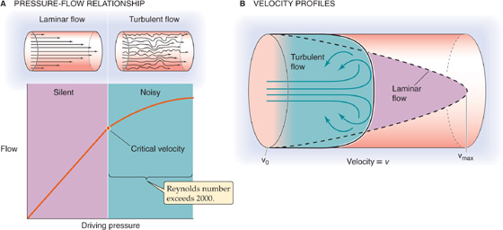
Figure 17-6 Laminar versus turbulent flow.
The critical parameter that determines when flow becomes turbulent is a dimensionless quantity called Reynolds number (Re), named after Osborne Reynolds: (See Note: Reynolds Number)
Blood flow is laminar when Re is below ~2000 and is mostly turbulent when Re exceeds ~3000. The terms in the numerator reflect disruptive forces produced by the inertial momentum in the fluid. Thus, turbulent blood flow occurs where r is large (e.g., aorta) or when is large (e.g., high cardiac output). Turbulent flow can also occur when a local decrease in vessel diameter (e.g., arterial stenosis) causes a local increase in . The term in the denominator of Equation 17-13, viscosity, reflects the cohesive forces that tend to keep the layers well organized. Therefore, a low viscosity (e.g., anemia—a low red blood cell count) predisposes to turbulence. When turbulence arises, the parabolic profile of the linear velocity across the radius of a cylinder becomes blunted (Fig. 17-6B).
The distinction between laminar and turbulent flow is clinically very significant. Laminar flow is silent, whereas vortex formation during turbulence sets up murmurs. These Korotkoff sounds are useful in assessing arterial blood flow in the traditional auscultatory method for determination of blood pressure. These murmurs are also important for diagnosis of vessel stenosis, vessel shunts, and cardiac valvular lesions (see the box titled Heart Murmurs and Arterial Bruits). Intense forms of turbulence may be detected not only as loud acoustic murmurs but also as mechanical vibrations or thrills that can be felt by touch.
Heart Murmurs and Arterial Bruits
Turbulence as blood flows across diseased heart valves creates murmurs that can be readily detected by auscultation with a stethoscope. The factors causing turbulence are the ones that increase Reynolds number: increases in vessel diameter or blood velocity and decreases in viscosity. Before the advent of sophisticated technology, such as cardiac ultrasonography, clinicians made a fine art of detecting these murmurs in an attempt to diagnose cardiac valvular disease. In general, it was appreciated that normal blood flow across normal heart valves is silent, although murmurs can occur with increased blood flow (e.g., exercise) and are not infrequently heard in young, thin individuals with dynamic circulations. The grading of heart murmurs helps standardize the cardiac examination from observer to observer. Thus, a grade 1 heart murmur is barely audible, grade 2 is one that is slightly more easily heard, and grades 3 and 4 are progressively louder. A grade 5 murmur is the loudest murmur that still requires a stethoscope to be heard. A grade 6 murmur is so loud that it can be heard with the stethoscope off the chest and is often accompanied by a thrill. The location, duration, pitch, and quality of a murmur aid in identifying the underlying valvular disorder.
Blood flowing through diseased arteries can also create a murmur or a thrill. By far the most common cause is atherosclerosis, which narrows the vessel lumen and thus increases velocity. In patients with advanced disease, these murmurs can be heard in virtually every major artery, most easily in the carotid and femoral arteries. Arterial murmurs are usually referred to as bruits.
Thus far we have considered blood flow to be steady and driven by a constant pressure generator. That is, we have been working with a mean blood flow and a mean driving pressure (the difference between the mean arterial and venous pressures). However, we are all aware that the heart is a pump of the “two-stroke” variety, with a filling and an emptying phase. Because both the left and right sides of the heart perform their work in a cyclic fashion, flow is pulsatile in both the systemic and pulmonary circulations.
The mean blood pressure in the large systemic arteries is ~95 mm Hg. This is a single, time-averaged value. In reality, the blood pressure cycles between a maximal systolic arterial pressure (~120 mm Hg) that corresponds to the contraction of the ventricle and a minimal diastolic arterial pressure (~80 mm Hg) that corresponds to the relaxation of the ventricle (Fig. 17-7). The difference between the systolic pressure and the diastolic pressure is pulse pressure. Note that the mean arterial pressure is not the arithmetic mean of systolic and diastolic values, which would be (120 + 80)/2 = 100 mm Hg in our example; rather, it is the area beneath the curve, which describes the pressure in a single cardiac cycle (Fig. 17-7, blue area) divided by the duration of the cycle. A reasonable value for the mean arterial pressure is 95 mm Hg.
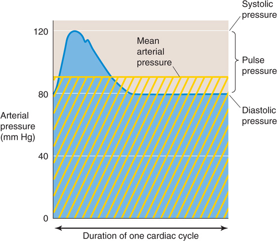
Figure 17-7 Time course of arterial pressure during one cardiac cycle. The area beneath the blue pressure curve, divided by the time of one cardiac cycle, is mean arterial pressure (horizontal yellow line). The yellow cross-hatched area is the same as the blue area.
Like arterial pressure, flow through arteries also oscillates with each heartbeat. Because both pressure and flow are pulsatile, and because the pressure and flow waves are not perfectly matched in time, we cannot describe the relationship between these two parameters by a simple Ohm’s law–like relationship (ΔP = F • R), which is analogous to a simple DC circuit in electricity. Rather, if we were to model pressure and flow in the circulatory system, we would have to use a more complicated approach, analogous to that used to understand AC electrical circuits. (See Note: Mechanical Impedance of Blood Flow)
Four factors help generate pressure in the circulation: gravity, compliance of the vessels, viscous resistance, and inertia.
Because gravity produces a hydrostatic pressure difference between two points whenever there is a difference in height (Δh; Equation 17-4), one must always express pressures relative to some reference h level. In cardiovascular physiology, this reference—zero height—is the level of the heart.
Whether the body is recumbent (i.e., horizontal) or upright (i.e., erect) has a tremendous effect on the intravascular pressure. In the horizontal position (Fig. 17-8A), where we assume that the entire body is at the level of the heart, we do not need to add a hydrostatic pressure component to the various intravascular pressures. Thus, the mean pressure in the aorta is 95 mm Hg, and—because it takes a driving pressure of ~5 mm Hg to pump blood into the end of the large arteries—the mean pressure at the end of the large arteries in the foot and head is 90 mm Hg. Similarly, the mean pressure in the large veins draining the foot and head is 5 mm Hg, and—because it takes a driving pressure of ~3 mm Hg to pump blood to the right atrium—the mean pressure in the right atrium is 2 mm Hg.
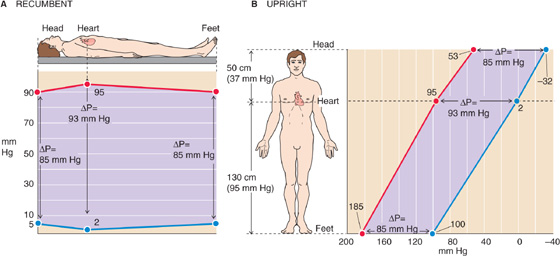
Figure 17-8 Arterial and venous pressures in the horizontal and upright positions. The pressures are different between A and B, but the driving pressures (ΔP) between arteries and veins (separation between red and blue lines, violet background) are the same.
When a 180-cm tall person is standing (Fig. 17-8B), we must add a 130-cm column of blood (the Δh between the heart and large vessels in the foot) to the pressure prevailing in the large arteries and veins of the foot. Because a water column of 130 cm is equivalent to 95 mm Hg, the mean pressure for a large artery in the foot will be 90 + 95 = 185 mm Hg, and the mean pressure for a large vein in the foot will be 5 + 95 = 100 mm Hg. On the other hand, we must subtract a 50-cm column of blood from the pressure prevailing in the head. Because a water column of 50 cm is equivalent to 37 mm Hg, the mean pressure for a large artery in the head will be 90 − 37 = 53 mm Hg, and the mean pressure for a large vein in the head will be 5 − 37 = −32 mm Hg. Of course, this “negative” value really means that the pressure in a large vein in the head is 32 mm Hg lower than the reference pressure at the level of the heart.
In this example, we have simplified things somewhat by ignoring the valves that interrupt the blood column. In reality, the veins of the limbs have a series of one-way valves that allow blood to flow only toward the heart. These valves act like a series of relay stations, so that the contraction of skeletal muscle around the veins pushes blood from one valve to another (see Chapter 22). Thus, veins in the foot do not “see” the full hydrostatic column of 95 mm Hg when the leg muscles pump blood away from the foot veins.
Although the absolute arterial and venous pressures are much higher in the foot than in the head, the ΔP that drives blood flow is the same in the vascular beds of the foot and head. Thus, in the horizontal position, the ΔP across the vascular beds in the foot or head is 90 − 5 = 85 mm Hg. In the upright position, the ΔP for the foot is 185 − 100 = 85 mm Hg, and for the head, 53 − (−32) = 85 mm Hg. Thus, gravity does not affect the driving pressure that governs flow. On the other hand, in “dependent” areas of the body (i.e., vessels “below” the heart in a gravitational sense), the hydrostatic pressure does tend to increase the transmural pressure (intravascular versus extravascular “tissue” pressure) and thus the diameter of distensible vessels. Because various anatomical barriers separate different tissue compartments, it is assumed that gravity does not appreciably affect this tissue pressure.
Until now, we have considered blood vessels to be rigid tubes, which, by definition, have fixed volumes. If we were to try to inject a volume of fluid into a truly rigid tube with closed ends, we could in principle increase the pressure to infinity without increasing the volume of the tube (Fig. 17-9A). At the other extreme, if the wall of the tube were to offer no resistance to deformation (i.e., infinite compliance), we could inject an infinite volume of fluid without increasing the pressure at all (Fig. 17-9B). Blood vessels lie between these two extremes; they are distensible but have a finite compliance (see Chapter 19). Thus, if we were to inject a volume of blood into the vessel, the volume of the vessel would increase by the same amount (ΔV), and the intravascular pressure would also increase (Fig. 17-9C). The ΔP accompanying a given ΔV is greater if the compliance of the vessel is lower. The relationship between ΔP and ΔV is a static property of the vessel wall and holds whether or not there is flow in the vessel. Thus, if we were to infuse blood into a patient’s blood vessels, the intravascular pressure would rise throughout the circulation, even if the heart were stopped.
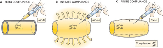
Figure 17-9 Compliance: changes in pressure with vessels of different compliances.
As we saw in Ohm’s law of hydrodynamics (see Equation 17-1), during steady flow down the axis of a tube (Fig. 17-2), the driving pressure (ΔP) is proportional to both flow and resistance. Viewed differently, if we want to achieve a constant flow, then the greater the resistance, the greater the ΔP that we must apply along the axis of flow. Of the four sources of pressure in the circulatory system, this ΔP due to viscous resistance is the only one that appears in Poiseuille’s law (see Equation 17-9).
For the most part, we have been assuming that the flow of blood as well as its mean linear velocity is steady. However, as we have already noted, blood flow in the circulation is not steady; the heart imparts its energy in a pulsatile manner, with each heartbeat. Therefore, in the aorta increases and reaches a maximum during systole and falls off during diastole. As we shall shortly see, these changes in velocity lead to compensatory changes in intravascular pressure.
The tradeoff between velocity and pressure reflects the conversion between two forms of energy. Although we generally state that fluids flow from a higher to a lower pressure, it is more accurate to say that fluids flow from a higher to a lower total energy. This energy is made up of both the pressure or potential energy and the kinetic energy (KE = ½ mv2). The impact of the interconversion between these two forms of energy is manifested by the familiar Bernoulli effect. As fluid flows along a horizontal tube with a narrow central region, which has half the diameter of the two ends, the pressure in the central region is actually lower than the pressure at the distal end of the tube (Fig. 17-10). How can the fluid paradoxically flow against the pressure gradient from the lower pressure central to the higher pressure distal region of the tube? We saw earlier that flow is the product of cross-sectional area and velocity (see Equation 17-8). Because the flow is the same in both portions of the tube, but the cross-sectional area in the center is lower by a factor of 4, the velocity in the central region must be 4-fold higher (Fig. 17-10, table at bottom). Although the blood in the central region has a lower potential energy (pressure = 60) than the blood at the distal end of the tube (pressure = 80), it has a 16-fold higher kinetic energy. Thus, the total energy of the fluid in the center exceeds that in the distal region, so that the fluid does indeed flow down the energy gradient.
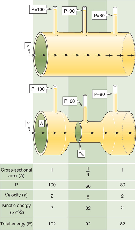
Figure 17-10 Bernoulli effect. For the top tube, which has a uniformly high radius, velocity (v) is uniform and transmural pressure (P) falls linearly with length. The bottom tube has the same upstream and downstream pressures but a constriction in the middle with a cross-sectional area that is only one fourth that of the two ends. Thus, velocity in the narrow portion must be 4-fold higher than it is at the ends. Although the total energy of fluid falls linearly along the tube, pressure is lower in the middle than at the distal end.
This example illustrates an interconversion between potential energy (pressure) and kinetic energy (velocity) in space because velocity changes along the length of a tube even though flow is constant. We will see in Chapter 22 that during ejection of blood from the left ventricle into the aorta, the flow and velocity of blood change with time at any point within the aorta. These changes in velocity contribute to the changes in pressure inside the aorta.
The Bernoulli effect has important practical implications for measurement of blood pressure with an open-tipped catheter. The pressure recorded with the open tip facing the flow is higher than the actual pressure by an amount corresponding to the kinetic energy of the oncoming fluid (Fig. 17-11). Conversely, the pressure recorded with the open tip facing away from the flow is lower than the actual pressure by an equal amount. The measured pressure is correct only when the opening is on the side of the catheter, perpendicular to the flow of blood.
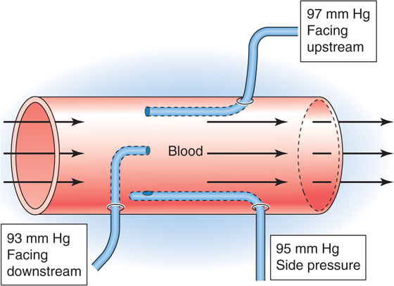
Figure 17-11 Effects of kinetic energy on the measurement of blood pressure with catheters.
One can record blood pressure anywhere along the circulation—inside a heart chamber, inside an artery, within a capillary, or within a vein. Clinicians are generally concerned with the intravascular pressure at a particular site (e.g., in a systemic artery) in reference to the barometric pressure outside the body and not with pressure differences between two sites.
The most direct approach for measurement of pressure is to introduce a needle or a catheter into a vessel and position the open tip at a particular site. In the first measurements of blood pressure ever performed, Stephen Hales in 1733 found that a column of blood from a presumably agitated horse rose to fill a brass pipe to a height of 3 meters. It was Poiseuille who measured blood pressure for the first time by connecting a mercury-filled U-tube to arteries through a tube containing a solution of saturated NaHCO3. In modern times, a saline-filled transmission or conduit system connects the blood vessel to a pressure transducer. In its most primitive form, a catheter was connected to a closed chamber, one wall of which was a deformable diaphragm. Nowadays, the pressure transducer is a stiff diaphragm bonded to a strain gauge that converts mechanical strain into a change in electrical resistance, capacitance, or inductance (Fig. 17-12). The opposite face of the diaphragm is open to the atmosphere, so that the blood pressure is referenced to barometric pressure. The overall performance of the system depends largely on the properties of the catheter and the strain gauge. The presence of air bubbles and a long or narrow catheter can decrease the displacement, velocity, and acceleration of the fluid in the catheter. Together, these properties determine overall performance characteristics such as sensitivity, linearity, damping of the pressure wave, and frequency response. To avoid problems with fluid transmission in the catheter, some high-fidelity devices employ a solid-state pressure transducer at the catheter tip.
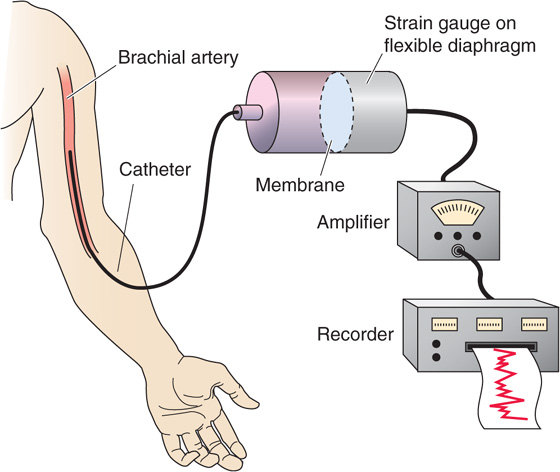
Figure 17-12 Direct method to determine blood pressure.
In catheterizations of the right side of the heart, the clinician begins by sliding a fluid-filled catheter into an antecubital vein and, while continuously recording pressure, advances the catheter tip into the superior vena cava, through the right atrium and the right ventricle, and past the pulmonary valve into the pulmonary artery. Eventually, the tip reaches and snugly fits into a smaller branch of the pulmonary artery, recording the pulmonary wedge pressure (see Chapter 22). The wedge pressure effectively measures the pressure downstream from the catheter tip, that is, the left atrial pressure.
In catheterizations of the left side of the heart, the clinician slides a catheter into the brachial artery or femoral artery, obtaining the systemic arterial blood pressure. From there, the catheter is advanced into the aorta, the left ventricle, and finally the left atrium.
Clinical measurements of venous pressure are typically made by inserting a catheter into the jugular vein. Because of the low pressures, these venous measurements require very sensitive pressure transducers or water manometers.
In the research laboratory, one can measure capillary pressure in exposed capillary beds by inserting a micropipette that is pressurized just enough (with a known pressure) to keep fluid from entering or leaving the pipette.
In clinical practice, one may measure arterial pressure indirectly by use of a manual sphygmomanometer (Fig. 17-13). An inextensible cuff containing an inflatable bag is wrapped around the arm (or occasionally the thigh). Inflation of the bag by means of a rubber squeeze-bulb to a pressure level above the expected systolic pressure occludes the underlying brachial artery and halts blood flow downstream. The pressure in the cuff, measured by means of a mercury or aneroid manometer, is then allowed to slowly decline (Fig. 17-13, diagonal red line). The physician can use either of two methods to monitor the blood flow downstream of the slowly deflating cuff. In the palpatory method, one detects the pulse as an indicator of flow by feeling the radial artery at the wrist. In the auscultatory method, the physician detects flow by using a stethoscope to detect the changing character of Korotkoff sounds over the brachial artery in the antecubital space.
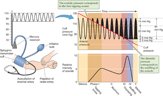
Figure 17-13 Sphygmomanometry. The clinician inflates the cuff to a pressure that is higher than the anticipated systolic pressure and then slowly releases the pressure in the cuff.
The palpatory method permits determination of the systolic pressure, that is, the pressure in the cuff below which it is just possible to detect a radial pulse. Because of limited sensitivity of the finger, palpation probably slightly underestimates systolic pressure. The auscultatory method permits the detection of both systolic and diastolic pressure. The sounds heard during the slow deflation of the cuff can be divided into five phases (Fig. 17-13). During phase I, there is a sharp tapping sound, indicating that a spurt of blood is escaping under the cuff when cuff pressure is just below systolic pressure. The pressure at which these taps are first heard closely represents systolic pressure. In phase II, the sound becomes a blowing or swishing murmur. During phase III, the sound becomes a louder thumping. In phase IV, as the cuff pressure falls toward the diastolic level, the sound becomes muffled and softer. Finally, in phase V, the sound disappears. Although some debate persists about whether the point of muffling or the point of silence is the correct diastolic pressure, most favor the point of muffling as being more consistent. Actual diastolic pressure may be somewhat overestimated by the point of muffling but underestimated by the point of silence.
Practical problems arise when a sphygmomanometer is used with children or obese adults or when it is used to obtain a measurement on a thigh. Ideally, one would like to use a pressure cuff wide enough to ensure that the pressure inside the cuff is the same as that in the tissue surrounding the artery. In 1967, the American Heart Association recommended that the pneumatic bag within the cuff be 20% wider than the diameter of the limb, extend at least halfway around the limb, and be centered over the artery. More recent studies indicate that accuracy and reliability improve when the pneumatic bag completely encircles the limb, as long as the width of the pneumatic bag is at least the limb diameter.
The spectrum of blood flow measurements in the circulation ranges from determinations of total blood flow (cardiac output) to assessment of flow within an organ or a particular tissue within an organ. Moreover, one can average blood flow measurements over time or record continuously. Examples of continuous recording include recordings of the phasic blood flow that occurs during the cardiac cycle or any other periodic event (e.g., breathing). We discuss both invasive and noninvasive approaches.
Invasive Methods These approaches require direct access to the vessel under study and are thus useful only in research laboratories. The earliest measurements of blood flow involved collecting venous outflow into a graduated cylinder and timing the collection with a stopwatch. This direct approach was limited to short time intervals to minimize blood loss and the resulting changes in hemodynamics. Blood loss could be avoided by ingenious but now antiquated devices that returned the blood to the circulation, in either a manual or a semiautomated fashion.
The most frequently used modern instruments for measurement of blood flow in the research laboratory are electromagnetic flowmeters based on the electromagnetic induction principle (Fig. 17-14). The vessel is placed in a magnetic field. According to Faraday’s induction law, moving any conductor (including an electrolyte solution, such as blood) at right angles to lines of the magnetic field generates a voltage difference between two points along an axis perpendicular to both the axis of the movement and the axis of the magnetic field. The induced voltage is

where B is the density of magnetic flux, is the average linear velocity, and D is the diameter of the moving column of blood.
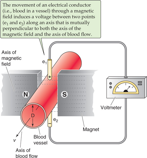
Figure 17-14 Electromagnetic flowmeter.
Ultrasound flowmeters employ a pair of probes, placed at two sites along a vessel. One probe emits an ultrasound signal, and the other records it. The linear velocity of blood in the vessel either induces a change in the frequency of the ultrasound signal (Doppler effect) or alters the transit time of the ultrasound signal. Both the electromagnetic and ultrasound methods measure linear velocity, not flow per se.
Noninvasive Methods The electromagnetic or ultrasonic flowmeters require the surgical isolation of a vessel. However, ultrasonic methods are also widely used transcutaneously on surface vessels in humans. This method is based on recording of the backscattering of the ultrasound signal from moving red blood cells. To the extent that the red blood cells move, the reflected sound has a frequency different from that of the emitted sound (Doppler effect). This frequency difference may thus be calibrated to measure flow. Plethysmographic methods are noninvasive approaches for measurement of changes in the volume of a limb or even of a whole person (see Chapter 27). Inflation of a pressure cuff enough to occlude veins but not arteries allows blood to continue to flow into (but not out of) a limb or an organ, so that the volume increases with time. The record of this rise in volume, as recorded by the plethysmograph, is a measure of blood flow.
With the exception of transcutaneous ultrasonography, the direct methods discussed for measurement of blood flow are largely confined to research laboratories. The next two sections include discussions of two indirect methods that clinicians use to measure mean blood flow.
The Fick method requires that a substance be removed from or added to the blood during its flow through an organ. The rate at which X passes a checkpoint in the circulation ( ) is simply the product of the rate at which blood volume passes the checkpoint (F) and the concentration of X in that blood:
The Fick principle is a restatement of the law of conservation of mass. The amount of X per unit time that passes a downstream checkpoint (B) minus the amount of X that passes an upstream checkpoint (A) must equal the amount of X added or subtracted per unit time (added/subtracted) between these two checkpoints (Fig. 17-15A):

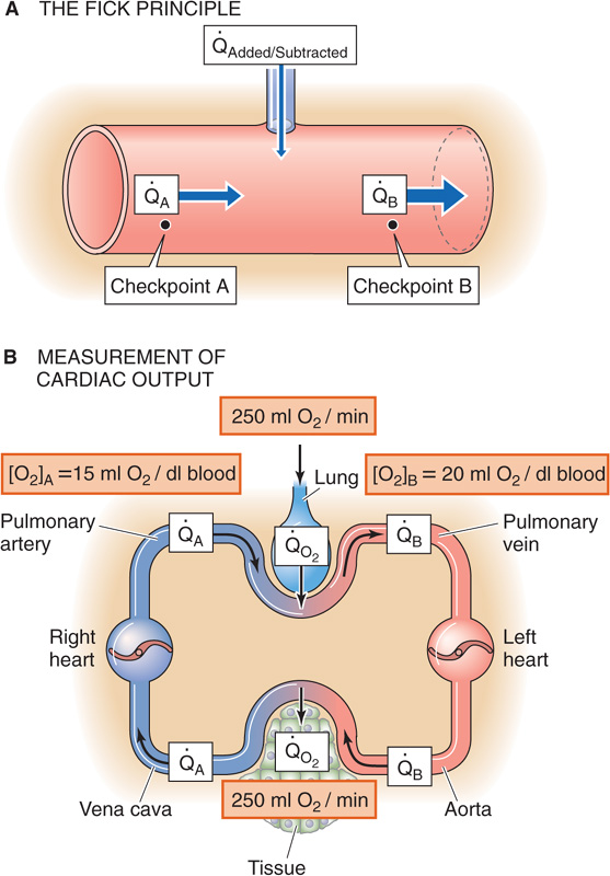
Figure 17-15 The Fick method to determine cardiac output.
added/subtracted is positive for the addition of X. If the volume flow is identical at both checkpoints, combining Equations 17-15 and 17-16 yields

We can calculate flow from the amount of X added or subtracted and the concentrations of X at the two checkpoints:
It is easiest to apply the Fick principle to the blood flow through the lungs, which is the cardiac output (Fig. 17-15B). The quantity added to the bloodstream is the O2 uptake (o2) by the lungs, which we obtain by measuring the subject’s O2 consumption. This value is typically 250 mL of O2 gas per minute. The upstream checkpoint is the pulmonary artery (point A), where the O2 content ([O2]A) is typically 15 mL of O2 per deciliter of blood. The sample for this checkpoint must reflect the O2 content of mixed venous blood, obtained by means of a catheter within the right atrium or the right ventricle or pulmonary artery. The downstream checkpoint is a pulmonary vein (point B), where the O2 content ([O2]B) is typically 20 mL of O2 per deciliter of blood. We can obtain the sample for this checkpoint from any systemic artery. Using these particular values, we calculate a cardiac output of 5 L/min:
The dye dilution method, inaugurated by G. N. Stewart in 1897 and extended by W. F. Hamilton in 1932, is a variation of the Fick procedure. One injects a known quantity of a substance (X) into a systemic vein (e.g., antecubital vein) at site A while simultaneously monitoring the concentration downstream at site B (Fig. 17-16A). It is important that the substance not leave the vascular circuit and that it is easy to follow the concentration, by either successive sampling or continuous monitoring. If we inject a single known amount (QX) of the indicator, an observer downstream at checkpoint B will see a rising concentration of X, which, after reaching its peak, falls off exponentially. Concentration measurements provide the interval (Δt) between the time the dye makes its first appearance at site B and the time the dye finally disappears there.
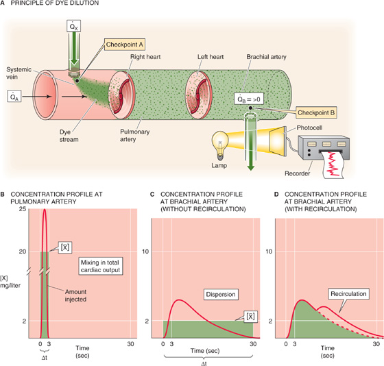
Figure 17-16 Dye dilution method to determine blood flow. In B, C, and D, the areas underneath the three red curves—as well as the three green areas—are all the same.
If site B is in the pulmonary artery, then the entire amount QX that we injected into the peripheral vein must pass site B during the interval Δt, carried by the entire cardiac output. We can deduce the average concentration [ ] during the interval Δt from the concentration-versus-time curve in Figure 17-16B. From the conservation of mass, we know that
Because the volume of blood (V) that flowed through the pulmonary artery during the interval Δt is, by definition, the product of cardiac output and the time interval (CO · Δt),
Note that the product Δt · is the area under the concentration-versus-time curve in Figure 17-16B. Solving for CO, we have
In practice, cardiologists monitor [X] in the brachial artery. Obviously, only a fraction of the cardiac output passes through a brachial artery; however, this fraction is the same as the fraction of QX that passes through the brachial artery. If we were to re-derive Equation 17-22 for the brachial artery, we would end up multiplying both the CO and QX terms by this same fraction. Therefore, even though only a small portion of both cardiac output and injected dye passes through any single systemic artery, we can still use Equation 17-22 to compute cardiac output with data from that artery.
Compared with the [X] profile in the pulmonary artery, the [X] profile in the brachial artery is not as tall and is more spread out, so that [] is smaller and Δt is longer. However, the product [] · Δt in the brachial artery—or any other systemic artery—is the same as in the pulmonary artery. Indocyanine green dye (cardiogreen) is the most common dye employed. Because the liver removes this dye from the circulation, it is possible to repeat the injections, after a sufficient wait, without progressive accumulation of dye in the plasma. Imagine that after we inject 5 mg of the dye, [] under the curve is 2 mg/L and Δt is 0.5 min. Thus,

A practical problem is that after we inject a marker into a systemic vein, blood moves more quickly through some pulmonary beds than others, so that the marker arrives at checkpoint B at different times. This process, known as dispersion, is the main cause of the flattening of the [X] profile in the brachial artery (Fig. 17-16C) versus the pulmonary artery (Fig. 17-16B). If we injected the dye into the left atrium and monitored it in the systemic veins, the dispersion would be far worse because of longer and more varied path lengths in the systemic circulation compared with the pulmonary circulation. In fact, the concentration curve would be so flattened that it would be difficult to resolve the area underneath the [X] profile.
A second practical problem with a closed circulatory system is that before the initial [X] wave has waned, recirculation causes the injected indicator to reappear for a second time in front of the sensor at checkpoint B (Fig. 17-16D). Extrapolation of the exponential decay of the first wave can correct for this problem.
The thermodilution technique is a convenient alternative approach to the dye technique. In this method, one injects a bolus of cold saline, and an indwelling thermistor is used to follow the dilution of these “negative calories” as a change of temperature at the downstream site. In the thermodilution technique, a temperature-versus-time profile replaces the concentration-versus-time profile. During cardiac catheterization, the cardiologist injects a bolus of cold saline into the right atrium and records the temperature change in the pulmonary artery. The distance between upstream injection and downstream recording site is kept short to avoid heat exchange in the pulmonary capillary bed. The advantages of this method are that (1) the injection of cold saline can be repeated without harm, (2) a single venous (versus venous and arterial) puncture allows access to both the upstream and the downstream sites, (3) less dispersion occurs because no capillary beds are involved, and (4) less recirculation occurs because of adequate temperature equilibration in the pulmonary and systemic capillary beds. A potential drawback is incomplete mixing, which may result from the proximity between injection and detection sites.
The methods used to measure regional blood flow are often called clearance methods, although the term here has a meaning somewhat different from its meaning in kidney physiology. Clearance methods are another application of the Fick principle, using the rate of uptake or elimination of a substance by an organ together with a determination of the difference in concentration of the indicator between the arterial inflow and venous outflow (i.e., the a-v difference). By analogy with Equation 17-18, we can compute the blood flow through an organ (F) from the rate at which the organ removes the test substance X from the blood (X) and the concentrations of the substance in arterial blood ([X]a) and venous blood ([X]v):
One can determine hepatic blood flow with use of BSP (bromosulphthalein), a dye that the liver almost completely clears and excretes into the bile (see Chapter 46). Here, X is the rate of removal of BSP from the blood, estimated as the rate at which BSP appears in the bile. [X]a is the concentration of BSP in a systemic artery, and [X]v is the concentration of BSP in the hepatic vein.
In a similar manner, one can determine renal blood flow with use of PAH (p-aminohippurate). The kidneys almost completely remove this compound from the blood and secrete it into the urine (see Chapter 34).
It is possible to determine coronary blood flow or regional blood flow through skeletal muscle from the tissue clearance of rapidly diffusing inert gases, such as the radioisotopes 133Xe and 85Kr.
Finally, one can use the rate of disappearance of nitrous oxide (N2O), a gas that is historically important as the first anesthetic, to compute cerebral blood flow.
A similar although qualitative approach is thallium scanning to assess coronary blood flow. Here one measures the uptake of an isotope by the heart muscle, rather than its clearance (see the box titled Thallium Scanning for Assessment of Coronary Blood Flow).
Thallium Scanning for Assessment of Coronary Blood Flow
Thallium is an ion that acts as a potassium analogue and enters cells through the same channels or transporters as K+ does. Active cardiac muscle takes up injected thallium Tl 201, provided there is adequate blood flow. Therefore, the rate of uptake of the 201Tl isotope by the heart is a useful qualitative measure of coronary blood flow. Complete 201Tl myocardial imaging is possible by two-dimensional scanning of the emitted γ-rays or by computed tomography for a three-dimensional image. Thus, in those portions of myocardial tissue supplied by stenotic coronary vessels, the uptake is slower, and these areas appear as defects on a thallium scan. Thallium scans are used to detect coronary artery disease during exercise stress tests.
Clinicians can use a variety of approaches to examine the cardiac chambers. Gated radionuclide imaging employs compounds of the γ-emitting isotope technetium Tc 99m, which has a half-life of 6 hours. After 99mTc is injected, a gamma camera provides imaging of the cardiac chambers. ECG gating (i.e., synchronization to a particular spot on the electrocardiogram) allows the apparatus to snap a picture at a specific part of the cardiac cycle and to sum these pictures up over many cycles. Because this method does not provide a high-resolution image, it yields only a relative ventricular volume. From the difference between the count at the maximally filled state (end-diastolic volume) and at its minimally filled state (end-systolic volume), the cardiologist can estimate the fraction of ventricular blood that is ejected during systole—the ejection fraction—which is an important measure of cardiac function. (See Note: 99mTc Scanning)
Angiography can accurately provide the linear dimensions of the ventricle, allowing the cardiologist to calculate absolute ventricular volumes. A catheter is threaded into either the left or the right ventricle, and saline containing a contrast substance (i.e., a chemical opaque to x-rays) is injected into the ventricle. This approach provides a two-dimensional projection of the ventricular volume as a function of time. In magnetic resonance imaging, one obtains a nuclear magnetic resonance (NMR) image of the protons in the water of the heart muscle and blood. However, because standard NMR requires long data acquisition times, it does not provide good time resolution.
Echocardiography, which exploits ultrasonic waves to visualize the heart and great vessels, can be used in two modes. In M-mode echocardiography (M is for motion), the technician places a single transducer in a fixed position on the chest wall and obtains a one-dimensional view of heart components. In the upper portion of Figure 17-17A, the ultrasonic beam transects the anterior wall of the right ventricle, the right ventricle, the septum, the left ventricle, the leaflets of the mitral valve, and the posterior wall of the left ventricle. The lower portion of Figure 17-17A shows the positions of the borders between these structures (x-axis) during a single cardiac cycle (y-axis) and thus how the size of the left ventricle—along the axis of the beam—changes with time. Of course, the technician can obtain other views by changing the orientation of the beam.
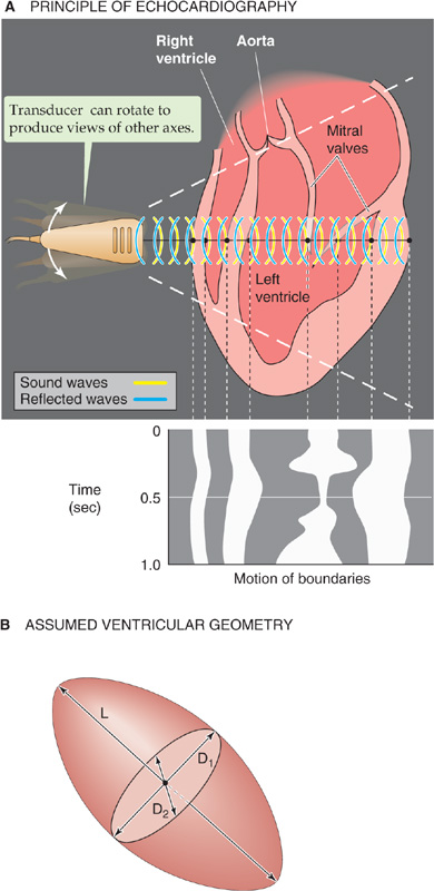
Figure 17-17 M-mode and two-dimensional echocardiography. In A, the tracing on the bottom shows the result of an M-mode echocardiogram (i.e., transducer in single position) during one cardiac cycle. The waves represent motion (M) of heart boundaries transected by a stationary ultrasonic beam. In two-dimensional echocardiography (upper panel), the probe rapidly rotates between the two extremes (broken lines), producing an image of a slice through the heart at one instant in time.
In two-dimensional echocardiography, the probe automatically and rapidly pivots, scanning the heart in a single anatomical slice or plane (Fig. 17-17A, area between the two broken lines) and providing a true cross section. This approach is therefore superior to angiography, which provides only a two-dimensional projection. Because cardiac output is the product of heart rate and stroke volume, one can calculate cardiac output from echocardiographic measurements of ventricular end-diastolic and end-systolic volume.
A problem common to angiography and M-mode echocardiography is that it is impossible to compute ventricular volume from a single dimension because the ventricle is not a simple sphere. As is shown in Figure 17-17B, the left ventricle is often assumed to be a prolate ellipse, with a long axis L and two short axes D1 and D2. To simplify the calculation and to allow ventricular volume to be computed from a single measurement, it is sometimes assumed that D1 and D2 are identical and that D1 is half of L. Unfortunately, use of this algorithm and just a single dimension, as provided by M-mode echocardiography, often yields grossly erroneous volumes. Use of two-dimensional echocardiography to sum information from several parallel slices through the ventricle, or from planes that are at a known angle to one another, can yield more accurate volumes. (See Note: Ventricular Volume from M-Mode Echocardiography)
In addition to ultrasound methods of angiography, magnetic resonance angiography is an application of magnetic resonance tomography to obtain two-dimensional images of slices of ventricular volumes or of blood vessels.
In contrast to standard echocardiography, Doppler echocardiography provides information on the velocity, direction, and character of blood flow, just as police radar monitors traffic. In Doppler echocardiography (as with police radar), most information is obtained with the beam parallel to the flow of blood. In the simplest application of Doppler flow measurements, one can continuously monitor the velocity of flowing blood in a blood vessel or part of the heart. On such a record, the x-axis represents time and the y-axis represents the spectrum of velocities of the moving red blood cells (i.e., different cells can be moving at different velocities). Flow toward the transducer appears above baseline, whereas flow away from the transducer appears below baseline. The intensity of the record at a single point on the y-axis (encoded by a gray scale or false color) represents the strength of the returning signal, which depends on the number of red blood cells moving at that velocity. Thus, Doppler echocardiography is able to distinguish the character of flow: laminar versus turbulent. Alternatively, at one instant in time, the Doppler technician can scan a region of a vessel or the heart, obtaining a two-dimensional, color-encoded map of blood velocities. If we overlay such two-dimensional Doppler data on a two-dimensional echocardiogram, which shows the position of the vessel or cardiac structures, the result is a color, flow-imaging Doppler echocardiogram (Fig. 17-18).
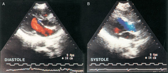
Figure 17-18 The colors, which encode the velocity of blood flow, are superimposed on a two-dimensional echocardiogram, which is shown in a gray scale. In A, blood moves through the mitral valve and into the left ventricle during diastole. Because blood is flowing toward the transducer, its velocity is encoded as red. In B, blood moves out of the ventricle and toward the aortic valve during systole. Because blood is flowing away from the transducer, its velocity is encoded as blue. (From Feigenbaum H: Echocardiography. In Braunwald E [ed]: Heart Disease: A Textbook of Cardiovascular Medicine, 5th ed. Philadelphia: WB Saunders, 1997.)
Finally, a magnetic resonance scanner can also be used in two-dimensional phase-contrast mapping to yield quantitative measurements of blood flow velocity.
Books and Reviews
Badeer HS: Hemodynamics for medical students. Adv Physiol Educ 2001; 25:44-52.
Caro CG, Pedley TJ, Schroter RC, Seed WA: The Mechanics of the Circulation. Oxford: Oxford University Press, 1978.
Lassen NA, Henriksen O, Sejrsen P: Indicator methods for measurement of organ and tissue blood flow. In Handbook of Physiology, Section 2: The Cardiovascular System, vol III, pp 21-63. Bethesda, MD: American Physiological Society, 1979.
Levine RA, Gillam LD, Weyman AE: Echocardiography in cardiac research. In Fozzard HA, Haber E, Jennings RB, et al (eds): The Heart and Cardiovascular System, pp 369-452. New York: Raven Press, 1986.
Rowland T, Obert P: Doppler echocardiography for the estimation of cardiac output with exercise. Sports Med 2002; 32:973-986.
Journal Articles
Coulter NA Jr, Pappenheimer JR: Development of turbulence in flowing blood. Am J Physiol 1949; 159:401-408.
Cournand A, Ranges HA: Catheterization of the right auricle. Proc Soc Exp Biol Med 1941; 46:462-466.
Hamilton WF, Moore JW, Kinsman JM, Spurling RG: Studies on the circulation. IV. Further analysis of the injection method and of changes in hemodynamics under physiological and pathological conditions. Am J Physiol 1932; 99:534-551.
Reynolds O: An experimental investigation of the circumstances which determine whether the motion of water shall be direct or sinusoid, and of the law of resistance in parallel channels. Philos Trans R Soc Lond B Biol Sci 1883; 174:935-982.
Thury A, van Langenhove G, Carlier SG, et al: High shear stress after successful balloon angioplasty is associated with restenosis and target lesion revascularization. Am Heart J 2002; 144:136-143.