CHAPTER 19

ARTERIES AND VEINS

Emile L. Boulpaep

THE ARTERIAL DISTRIBUTION AND VENOUS COLLECTION SYSTEMS

Hemodynamics is the study of the physical laws of blood circulation. It therefore addresses the properties of both the “content” (i.e., blood) and the “container” (i.e., blood vessels). In Chapter 18, we discussed the properties of the blood. This chapter is primarily concerned with the properties of the blood vessels. The circulation is not a system of rigid tubes. Moreover, the anatomy and functions of the various segments of the vasculature differ greatly from one to another. Because the function of the circulation is to carry substances all over the body, the circulatory system branches out into a network of billions of tiny capillaries. We can think of the arteries as a distribution system, the microcirculation as a diffusion and filtration system, and the veins as a collection system.

Physical properties of vessels closely follow the level of branching in the circuit

The aorta branches out into billions of capillaries that ultimately regroup into a single vena cava (Fig. 19-1, panel 1). At each level of arborization of the peripheral circulation, the values of several key parameters vary dramatically:

1. Number of vessels at each level of arborization

2. Radius of a typical individual vessel

3. Aggregate cross-sectional area of all vessels at that level

4. Mean linear velocity of blood flow within an individual vessel

5. Flow (i.e., volume/second) through a single vessel

6. Relative blood volume (i.e., the fraction of the body’s total blood volume present in all vessels of a given level)

7. Circulation (i.e., transit) time between two points of the circuit

8. Pressure profile along that portion of the circuit

9. Structure of the vascular walls

10. Elastic properties of the vascular walls

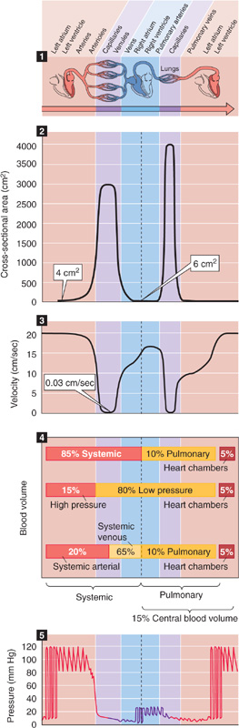
Figure 19-1 Profile of key parameters along the cardiovascular system. Panel 1 (top) shows branching of the cardiovascular system, from left side to right side of heart and back to left. Panel 2 shows the variation of aggregate cross-sectional area of all vessels at any level of branching. Panel 3 shows how mean linear velocity of blood varies in typical vessels. Panel 4 shows ways of grouping blood volume in various compartments. Panel 5 shows profile of blood pressure, with superimposed oscillations that represent variations in time.

We discuss items 1 to 5 in this section and items 6 to 8 in the following two sections. Items 9 and 10 are the subject of the second subchapter.

The number of vessels at a particular level of arborization (Table 19-1) increases enormously from a single aorta to ~104 small arteries, ~107 arterioles, and finally ~4 × 1010 capillaries. However, only about one fourth of all capillaries are normally open to flow at rest. Finally, all of the blood returns to a single vessel where the superior and inferior venae cavae join.

Table 19-1 Key Systemic Vascular Parameters That Vary with Arborization

The radius of an individual vessel (ri; Table 19-1) declines as a result of the arborization, decreasing from 1.1 cm in the aorta to a minimum of ~3 μm in the smallest capillaries. Because the cross-sectional area of an individual vessel is proportional to the square of the radius, this parameter decreases even more precipitously.

The aggregate cross-sectional area (Table 19-1) at any level of branching is the sum of the single cross-sectional areas of all parallel vessels at that level of branching. That is, it is the area that you would see if you sliced through all of the vessels at the same level of branching in panel 1 of Figure 19-1.

A fundamental law of vessel branching is that at each branch point, the combined cross-sectional area of daughter vessels exceeds the cross-sectional area of the parent vessel. In this process of bifurcation, the steepest increase in total cross-sectional area occurs in the microcirculation (Fig. 19-1, panel 2). A typical microcirculation in the smooth muscle and submucosa of the intestine (Fig. 19-2) encompasses a first-order arteriole, several orders of progressively smaller arterioles, capillaries, several orders of venules into which the capillaries empty, and eventually a first-order venule. In humans, the maximum cross-sectional area occurs not at the level of the capillaries but at the “postcapillary” (i.e., fourth-order) venules. Because of anastomoses among capillaries, capillaries only slightly outnumber fourth-order venules, whereas the cross-sectional unit area of each venule is appreciably greater than the area of a capillary. Assuming that only a quarter of the capillaries are usually open, the peak aggregate cross-sectional area of these postcapillary venules can be ~1000-fold greater than the cross section of the parent artery (e.g., aorta), as shown in panel 2 of Figure 19-1.

Figure 19-2 Branching in a typical microcirculation, that of the smooth muscle and submucosa of the intestine. r, radius.

The profile of the mean linear velocity of flow () along a vascular circuit (Fig. 19-1, panel 3) is roughly a mirror image of the profile of the total cross-sectional area. According to the principle of continuity, which is an application of conservation of mass, total volume flow of blood must be the same at any level of arborization. Indeed, as we make multiple vertical slices along the abscissa of panel 1 in Figure 19-1, the aggregate flow for each slice is the same:

As a consequence, must be minimal in the postcapillary venules (~0.03 cm/s), where Atotal is maximal. Conversely, is maximal in the aorta (~20 to 50 cm/s). Thus, both Atotal and values range ~1000-fold from the aorta to the capillaries but are inversely related to one another. The vena cava, with a cross-sectional area ~50% larger than that of the aorta, has a mean linear velocity that is about one third less.

Single-vessel flow, in contrast to total flow, ranges by approximately 10 orders of magnitude. In the aorta, the flow is ~83 mL/s, the same as the cardiac output (~5 L/min). When about 25% of the capillaries are open, a typical capillary has a mean linear velocity of 0.03 cm/s and a flow of 8 × 10−9 mL/s (8 pL/s)—10 orders of magnitude less than the flow in the aorta. Within the microcirculation, single-vessel flow has considerable range. At one extreme, a first-order arteriole (ri, ~30 μm) may have a flow of 20 × 10−6 mL/s. At the other, the capillaries that are closed at any given time have zero flow.

Most of the blood volume resides in the systemic veins

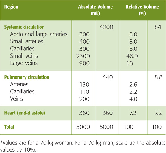
The body’s total blood volume (V) of about 5 L (see Table 5-1) is not uniformly distributed along the x-axis of panel 1 in Figure 19-1. At any level of branching, the total blood volume is the sum of the volumes of all parallel branches. Table 19-2 summarizes—for a hypothetical 70-kg woman—the distribution of total blood volume expressed as both absolute blood volumes and relative blood volumes (percentage of total blood volume). Panel 4 in Figure 19-1 summarizes four useful ways of grouping these volumes.

Table 19-2 Distribution of Blood Volume*

First, we can divide the blood volume into the systemic circulation (where ~85% of blood resides), the pulmonary circulation (~10%), and the heart chambers (~5%). The pulmonary blood volume is quite adjustable (i.e., it can be much higher than 10%) and is carefully regulated.

Second, as can be seen in the next section, we can divide blood volume into what is contained in the high-pressure system (~15%), the low-pressure system (~80%), and the heart chambers (~5%).

Third, we can group the blood volumes into those in the systemic venous system versus the remainder of the circulation. Of the 85% of the total blood volume that resides in the systemic circulation, about three fourths—or 65% of the total—is on the venous side, particularly in the smaller veins. Thus, the venous system acts as a volume reservoir. Changes in the diameters of veins have a major impact on the amount of blood they contain. For example, an abrupt increase in venous capacity causes pooling of blood in venous segments and may lead to syncope (i.e., fainting).

We can also use a fourth approach for grouping of blood volumes—divide the blood into the central blood volume (volumes of heart chambers and pulmonary circulation) versus the rest of the circulation. This central blood volume is very adjustable, and it constitutes the filling reservoir for the left side of the heart. Left-sided heart failure can cause the normally careful regulation of the central blood volume to break down.

The circulation time is the time required for a bolus of blood to travel either across the entire length of the circulation or across a particular vascular bed. Total circulation time (the time to go from left to right across panel 1 in Fig. 19-1) is ~1 minute. Circulation time across a single vascular bed (e.g., coronary circulation) may be as short as 10 seconds. Circulation times may be obtained in humans by injection of a substance such as ether into an antecubital vein and measurement of the time to its appearance in the lung (4 to 8 seconds) or by injection of a bitter or sweet substance and measurement of the time to the perception of taste in the tongue (10 to 18 seconds). Although, in the past, circulation time was used clinically as an index of cardiac output, the measurement has little physiological significance. The rationale for determination of circulation time was that a shortening of circulation time could signify an improvement of cardiac output. However, the interpretation is more complicated because circulation time is actually the ratio of blood volume to blood flow:

Changes in circulation time may thus reflect changes in volume as well as in flow. For instance, a patient in heart failure may have a decreased cardiac output (i.e., F) or an increased blood volume (i.e., V), both of which would contribute to an elevation of transit time.

The intravascular pressures along the systemic circuit are higher than those along the pulmonary circuit

Panel 5 in Figure 19-1 shows the profile of pressure along the systemic and pulmonary circulations. Pressures are far higher in the systemic than in the pulmonary circulation. Although the cardiac outputs of the left and right sides of the heart are the same in the steady state, the total resistance of the systemic circulation is far higher than that of the pulmonary circulation (see Chapter 31). This difference explains why the upstream driving pressure averages ~95 mm Hg in the systemic circulation but only ~15 mm Hg in the pulmonary circulation. Table 19-3 summarizes typical mean values at key locations in the circulation. In both the systemic and pulmonary circulations, the systolic and diastolic pressures decay downstream from the ventricles (Fig. 19-3). The instantaneous pressures vary throughout each cardiac cycle for much of the circulatory system (Fig. 19-1, panel 5). In addition, the systemic venous and pulmonary pressures vary with the respiratory cycle, and venous pressure in the lower limbs varies with the contraction of skeletal muscle.

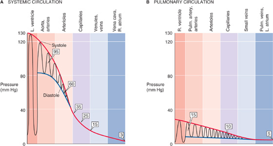
Figure 19-3 Pressure profiles along systemic and pulmonary circulations. In A and B, the oscillations represent variations in time, not distance. Boxed numbers indicate mean pressures.

Table 19-3 Mean Pressures in the Systemic and Pulmonary Circulations

As noted earlier, the circulation can be divided into a high-pressure and a low-pressure system. The high-pressure system extends from the left ventricle in the contracted state all the way to the systemic arterioles. The low-pressure system extends from the systemic capillaries, through the rest of the systemic circuit, into the right side of the heart, and then through the pulmonary circuit into the left side of the heart in the relaxed state. The pulmonary circuit, unlike the systemic circuit, is entirely a low-pressure system; mean arterial pressures normally do not exceed 15 mm Hg, and the capillary pressures do not rise above 10 mm Hg.

Under normal conditions, the steepest pressure drop in the systemic circulation occurs in arterioles, the site of greatest vascular resistance

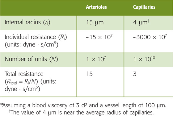
If we assume for simplicity’s sake that the left side of the heart behaves like a constant pressure generator of 95 mm Hg and the right side of the heart behaves like a constant pressure generator of 15 mm Hg, it is the resistance of each vascular segment that determines the profile of pressure fall between the upstream arterial and downstream venous ends of the circulation. In particular, the pressure difference between two points along the axis of the vessel (i.e., the driving pressure difference, ΔP) depends on flow and resistance: ΔP = F · R. According to Poiseuille’s law, the resistance (Ri) of an individual, unbranched vascular segment is inversely proportional to the fourth power of the radius (see Chapter 17). Thus, the pressure drop between any two points along the circuit depends critically on the diameter of the vessels between these two points. However, the steepest pressure drop (ΔP/Δx) does not occur along the capillaries, where vessel diameters are smallest, but rather along the precapillary arterioles. Why? The aggregate resistance contributed by vessels of a particular order of arborization depends not only on their average radius but also on the number of vessels in parallel. The more vessels in parallel, the smaller the aggregate resistance (see Equation 17-3). Although the resistance of a single capillary exceeds that of a single arteriole, capillaries far outnumber arterioles (Table 19-4). The result is that the aggregate resistance is larger in the arterioles, and this is where the steepest ΔP occurs. (See Note: Relative Resistance of Arterioles vs Capillaries)

Table 19-4 Estimates of Total Arteriolar and Capillary Resistances*

Local intravascular pressure depends on the distribution of vascular resistance

We have just seen that the ΔP between an upstream checkpoint and a downstream checkpoint depends on the resistance between these points. What determines the absolute pressure at some location between the two checkpoints? To answer this question, we need to know not only the upstream arterial and downstream venous pressures but also the distribution of resistance between the two checkpoints. A good example to explain this concept is the distribution of resistance and pressure in the systemic microvasculature. Just how the upstream pressure in the arteriole and the downstream pressure in the venule affect the pressure at the midpoint of the capillary (Pc) depends on the relative size of the upstream and downstream resistances. For the simple circuit illustrated in Figure 19-4A: (See Note: Derivation of Equation for Mid-Capillary Pressure)

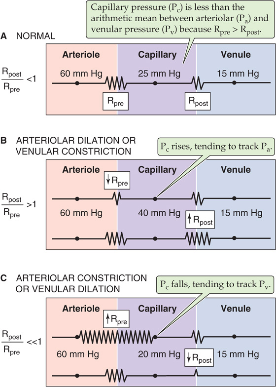
Figure 19-4 Effect of precapillary and postcapillary resistances on capillary pressure.

Pa is arteriolar pressure, Pv is venular pressure, Rpre is precapillary resistance upstream of the capillary bed, and Rpost is postcapillary resistance downstream of the capillary.

From this equation, we can draw three conclusions about local microvascular pressure. First, even though arteriolar pressure is 60 mm Hg and venular pressure is 15 mm Hg in our example (Table 19-3), capillary pressure is not necessarily 37.5 mm Hg, the arithmetic mean. According to Equation 19-3, Pc would be the arithmetic mean only if the precapillary and postcapillary resistances were identical (i.e., Rpost/Rpre = 1). The finding that Pc is ~25 mm Hg in most vascular beds (Fig. 19-4A) implies that Rpre exceeds Rpost (i.e., Rpost/Rpre > 1). Under normal conditions in most microvascular beds, Rpost/Rpre ranges from 0.2 to 0.4.

The second implication of Equation 19-3 is that as long as the sum (Rpre + Rpost) is constant, reciprocal changes in Rpre and Rpost would not alter the total resistance of the circuit and would therefore leave both Pa and Pv constant. However, as Rpost/Rpre increases, Pc would increase, thereby approaching Pa (Fig. 19-4B). Conversely, as Rpost/Rpre decreases, Pc would decrease, approaching Pv (Fig. 19-4C). This conclusion is also intuitive. If we reduced Rpre to zero (but increased Rpost to keep Rpost + Rpre constant), no pressure drop would occur along the precapillary vessels, and Pc would be the same as Pa. Conversely, if Rpost were zero, Pc would be the same as Pv.

The third conclusion from Equation 19-3 is that depending on the value of Rpost/Rpre, Pc may be more sensitive to changes in arteriolar than in venular pressure, or vice versa. For example, when the ratio Rpost/Rpre is low (i.e., Rpre > Rpost, as in Fig. 19-4A or 19-4C), capillary pressure tends to follow the downstream pressure in large veins. This phenomenon explains why standing may cause the ankles to swell. The elevated pressure in large leg veins translates to an increased Pc, which, as discussed later, leads to increased transudation of fluid from the capillaries into the interstitial spaces (see Chapter 20). It also explains why elevation of the feet, which lowers the pressure in the large veins, reverses ankle edema.

Vascular resistance varies in time and depends critically on the action of vascular smooth muscle cells. The major site of control of vascular resistance in the systemic circulation is the terminal small arteries (or feed arteries) and arterioles. Figure 19-5 illustrates the effect of vasoconstriction or vasodilation on the pressure profile. Whereas the overall ΔP between source and endpoint may not vary appreciably during a change in vascular resistance, the shape of the local pressure profile may change appreciably. Thus, during arteriolar constriction, the pressure drop between two points along the circuit (i.e., axial pressure gradient, ΔP/Δx) is steep and concentrated at the arteriolar site (Fig. 19-5, green curve). During arteriolar dilation, the gradient is shallow and more spread out (Fig. 19-5, violet curve).

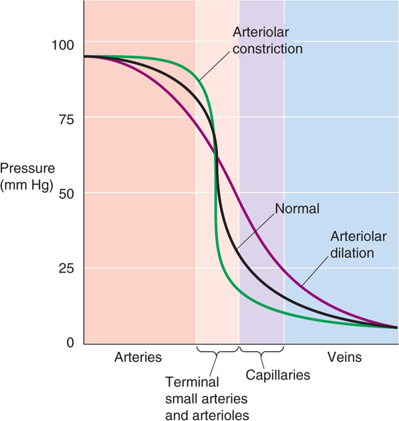
Figure 19-5 Pressure profiles during vasomotion. In this example, we assume that constriction or dilation of terminal arteries and arterioles does not affect the overall driving pressure (ΔP) between aorta and vena cava. This assumption is reasonable in two cases: (1) vasoconstriction or vasodilation is confined to a single parallel vascular bed (e.g., one limb) and does not substantially change total peripheral resistance; and (2) even if total peripheral resistance does change, the cardiac pump could still maintain constant systemic arterial and venous pressures.

Although the effects of vasoconstriction and vasodilation are greatest in the local arterioles (lighter red band in Fig. 19-5), the effects extend both upstream (darker red band) and downstream (purple and blue bands) from the site of vasomotion because the pressure profile along the vessel depends on the resistance profile. Thus, if one vascular element contributes a greater fraction of the total resistance, a greater fraction of the pressure drop will occur along that element.

ELASTIC PROPERTIES OF BLOOD VESSELS

Blood vessels are elastic tubes

The wall of blood vessels consists of three layers: the intima, the media, and the adventitia. Capillaries, which have only an intimal layer of endothelial cells resting on a basal lamina, are the exception. Regardless of the organization of layers, one can distinguish four building blocks that make up the vascular wall: endothelial cells, elastic fibers, collagen fibers, and smooth muscle cells. Figure 19-6 shows how the relative abundance of these components varies throughout the vascular circuit. In addition to these principal components, fibroblasts, nerve endings, and blood cells invade the intima; other extracellular components (e.g., proteoglycans) may also be present.

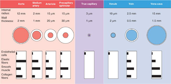
Figure 19-6 Structure of blood vessels. The values for medium arteries, arterioles, venules, and veins are merely illustrative because the dimensions can range widely. The drawings of the vessels are not to scale.

Endothelial cells form a single, continuous layer that lines all vascular segments. Junctional complexes keep the endothelial cells together in arteries but are less numerous in veins. The organization of the endothelial cell layer in capillaries varies greatly, depending on the organ (see Chapter 20). The glomus bodies in the skin and elsewhere are unusual in that their “endothelial cells” exist in multiple layers of cells called myoepithelioid cells. These glomus bodies control small arteriovenous shunts or anastomoses (see Chapter 24).

Elastic fibers are a rubber-like material that accounts for most of the stretch of vessels at normal pressures as well as the stretch of other tissues (e.g., lungs). Elastic fibers have two components: a core of elastin and a covering of microfibrils. The elastin core consists of a highly insoluble polymer of elastin, a protein rich in nonpolar amino acids (i.e., glycine, alanine, valine, proline). After being secreted into the extracellular space, the elastin molecules remain in a randomcoil configuration. They covalently cross-link and assemble into a highly elastic network of fibers, capable of stretching more than 100% under physiological conditions. The microfibrils, which are composed of glycoproteins and have a diameter of ~10 nm, are similar to those found in the extracellular matrix in other tissues. In arteries, elastic fibers are arranged as concentric, cylindrical lamellae. A network of elastic fibers is abundant everywhere except in the true capillaries, in the venules, and in the aforementioned arteriovenous anastomoses.

Collagen fibers constitute a jacket of far less extensible material than the elastic fibers, like the fabric woven inside the wall of a rubber hose. Collagen can be stretched only 3% to 4% under physiological conditions. The basic unit of the collagen fibers in blood vessels is composed of type I and type III collagen molecules, which are two of the fibrillar collagens. After being secreted, these triple-helical molecules assemble into fibrils that may be 10 to 300 nm in diameter; these in turn aggregate into collagen fibers that may be several microns in diameter and are visible with a light microscope. Collagen fibers are present throughout the circulation except in the capillaries. Collagen and elastic fibers form a network that is arranged more loosely toward the inner surface of the vessel than at the outer surface. Collagen fibers are usually attached to the other components of the vascular wall with some slack, so that they are normally not under tension. Stretching of these other components may take up the slack on the collagen fibers, which may then contribute to the overall tension.

Vascular smooth muscle cells (VSMCs) are also present in all vascular segments except the capillaries. In elastic arteries, VSMCs are arranged in spirals with pitch varying from nearly longitudinal to nearly transverse-circular; whereas in muscular arteries, they are arranged either in concentric rings or as helices with a low pitch. Relaxed VSMCs do not contribute appreciably to the elastic tension of the vascular wall, which is mainly determined by the elastin and collagen fibers. VSMCs exert tension primarily by means of active contraction (see Chapter 9).

Because of the elastic properties of vessels, the pressure-flow relationship of passive vascular beds is nonlinear

Because blood vessels are elastic, we must revise our concept of blood flow, which was based on Poiseuille’s law for rigid tubes (see Chapter 17). Poiseuille’s law predicts a linear pressure-flow relationship (Fig. 19-7A, broken line). However, in reality, the pressure-flow relationship is markedly nonlinear in an in vivo preparation of a vascular bed (Fig. 19-7A, red curve). Starting at the foot of the red curve at a driving pressure of about 6 mm Hg, we see that the curve rises more steeply as the driving pressure increases. The reason is that increase of the driving pressure (i.e., axial pressure gradient) also increases the transmural pressure, causing the vessel to distend. Because radius increases, resistance falls and flow rises more than it would in a rigid tube. Thus, the plot curves upward. The elastic properties of vessels are the major cause of such nonlinear pressure-flow relationships in vascular beds exhibiting little or no “active tension.”

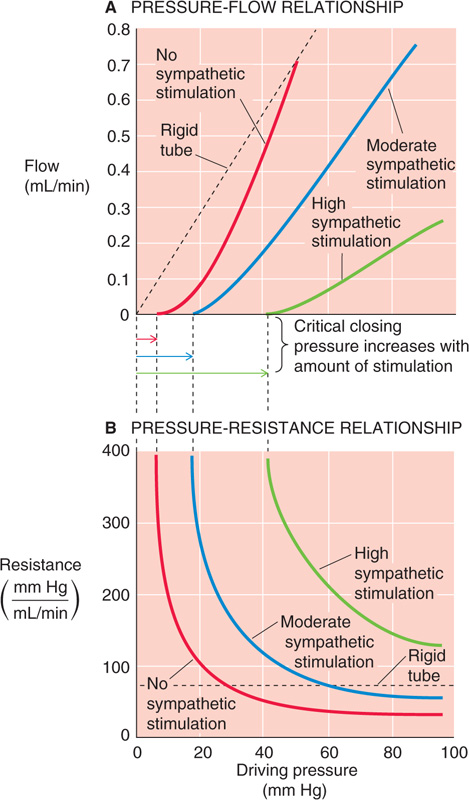
Figure 19-7 Nonlinear relationships among pressure, flow, and resistance. (See Note: Nonlinear Relationships among Pressure, Flow, and Resis-tance)

As driving pressure—and thus transmural pressure—increases, vessel radius increases as well, causing resistance (see Chapter 17) to fall (Fig. 19-7B, red curve). Conversely, resistance increases toward infinity when driving pressure falls. In Poiseuille’s case, of course, resistance would be constant (Fig. 19-7B, broken line), regardless of the driving pressure. Although many vascular beds behave like the red curves in Figure 19-7A and B, we will see in Chapter 24 that some are highly regulated (i.e., active tension varies with pressure). These special circulations therefore exhibit a pressure-flow relationship that differs substantially from that of a system of elastic tubes.

Contraction of smooth muscle halts blood flow when driving pressure falls below the critical closing pressure

As we have already seen, at low values of driving pressure, resistance rises abruptly toward infinity (Fig. 19-7B, red curve). Viewed differently, flow totally ceases when the pressure falls below about 6 mm Hg, the critical closing pressure (Fig. 19-7A, red curve). The stoppage of flow occurs because of the combined action of elastic fibers and active tension from VSMCs. Graded increases in active tension—produced, for example by sympathetic stimulation—shift the pressure-flow relationship to the right and decrease the slope (Fig. 19-7A, blue and green curves), reflecting an increase in resistance over the entire pressure range (Fig. 19-7B, blue and green curves). The critical closing pressure also shifts upward with increasing degrees of vasomotor tone. This phenomenon is important in hypotensive shock, where massive vasoconstriction occurs—in an attempt to raise arterial pressure—and critical closing pressures rise to 40 mm Hg or more. As a result, blood flow can stop completely in the limb of a patient in hypotensive shock, despite the persistence of a finite, albeit small, pressure difference between the main artery and vein.

Elastic and collagen fibers determine the distensibility and compliance of vessels

Arteries and veins must withstand very different transmural pressures in vivo (Table 19-3). Moreover, their relative blood volumes respond in strikingly different ways to increases in transmural pressure (Fig. 19-8). Arteries have a low volume capacity but can withstand large transmural pressure differences. In contrast, veins have a large volume capacity (and are thus able to act as blood reservoirs) but can withstand only small transmural pressure differences.

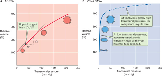
Figure 19-8 Compliance of blood vessels. In A and B, relative volume of 100% represents fully relaxed volume.

The abundance of structural elements in the vascular walls also differs between arteries and veins (Fig. 19-6). These disparities contribute to differences in the elastic behavior of arteries and veins. We can study the elastic properties of an isolated blood vessel either by recording the “static” volume change produced by pressurizing the vessel to different levels or, conversely, by recording the “static” pressure change produced by filling the vessel with liquid to different volumes. After the pressure or volume is altered experimentally, it is important to wait until the vessel has finished responding (i.e., it becomes static) before the measurements are recorded.

The volume distensibility expresses the elastic properties of blood vessels. Three measurements are useful for assessment of distensibility. First, the absolute distensibility is the change in volume for a macroscopic step change in pressure, ΔV/ΔP. Second, because the unstretched size varies among vessels, it is preferable to normalize the volume change to the initial, unstretched volume (V0) and thus to use a normalized distensibility instead:

This ratio is a measurement of the fractional change in volume with a given step in pressure. Third, the most useful index of distensibility is compliance (C), which is the slope of the tangent to any point along the pressure-volume diagram in Figure 19-8:

Here, the ΔV and ΔP values are minute displacements. The steeper the slope of a pressure-volume diagram, the greater the compliance (i.e., the easier it is to increase volume). In Figure 19-8, the slope—and thus the compliance—decreases with increasing volumes. For such a nonlinear relationship, this variable compliance is the slope of the tangent to the curve at any point. Thus, a compliance reading should always include the transmural pressure or the volume at which it was made. Similar principles apply to the compliance of airways in the lung (see Chapter 27).

Differences in compliance cause arteries to act as resistors and veins to act as capacitors

As we increase transmural pressure, arteries increase in volume. As they accommodate the volume of blood ejected with every heartbeat, large, muscular systemic arteries (e.g., femoral artery) increase in radius by about 10%. This change for a typical muscular artery is much smaller than the distention that one would observe for elastic arteries (e.g., aorta), which have fewer layers of smooth muscle and are not under nervous control. The higher compliance of elastic arteries is evident in the pressure-volume diagram in Figure 19-8A—obtained after the smooth muscle is relaxed. The compliance of a relaxed elastic artery is substantial. Increase of the transmural pressure from 0 to 100 mm Hg (near the normal, mean arterial pressure) increases relative volume by ~180%. With further increases in pressure and diameter, compliance decreases only modestly. For example, increase of transmural pressure from 100 to 200 mm Hg increases relative volume by a further ~100 percentage points. Thus, arteries are properly constituted for development and withstanding of high transmural pressures. Because an increase in pressure raises the radius only modestly under physiological conditions, paticularly in muscular arteries, the resistance of the artery (inversely proportional to r4) does not fall markedly. Because muscular arteries have a rather stable resistance, they are sometimes referred to as resistance vessels.

Veins behave very differently. The pressure-volume diagram of a vein (Fig. 19-8B) shows that compliance is extremely high—far higher than for elastic arteries—at least in the low-pressure range. For a relaxed vein, a relatively small increase of transmural pressure from 0 to 10 mm Hg increases volume by ~200%. This high compliance in the low-pressure range is not due to a property of the elastic fibers. Rather, it reflects a change in geometry. At pressures below 6 to 9 mm Hg, the vein’s cross section is ellipsoidal. A small rise in pressure causes the vein to become circular, without an increase in perimeter but with a greatly increased cross-sectional area. Thus, in their normal pressure range (Table 19-3), veins can accept relatively large volumes of blood with little buildup of pressure. Because they act as volume reservoirs, veins are sometimes referred to as capacitance vessels. The true distensibility or compliance of the venous wall—related to the increase in perimeter produced by pressures above 10 mm Hg—is rather poor, as shown by the flat slope at higher pressures in Figure 19-8B.

How do veins and elastic arteries compare in response to a sudden increase in volume (ΔV)? When the heart ejects its stroke volume into the aorta, the intravascular pressure increases modestly, from 80 to 120 mm Hg. This change in intravascular pressure—also known as the pulse pressure (see Chapter 17)—is the same as the change in transmural pressure. We have already seen that venous compliance is low in this “arterial” pressure range. Thus, if we were to challenge a vein with a sudden increase in volume (ΔV) in the arterial pressure range, the increase in transmural pressure (ΔP) would be much higher than in an artery of equal size. This is indeed the case when a surgeon uses a saphenous vein segment in a coronary artery bypass graft and anastomoses the vein between two sites on a coronary artery, forming a bypass around an obstructed site.

Changes in the volume of vessels during the cardiac cycle are due to changes in radius rather than length. During ejection of blood during systole, the length of the thoracic aorta may increase by only about 1%. (See Note: Changes in Vessel Volume)

Laplace’s law describes how tension in the vessel wall increases with transmural pressure

Because compliance depends on the elastic properties of the vessel wall, the discussion here focuses on how an external force deforms elastic materials. When the force vanishes, the deformation vanishes, and the material returns to its original state. The simplest mechanical model of a linearly elastic solid is a spring (Fig. 19-9A). The elongation ΔL is proportional to the force (F), according to Hooke’s law: k is a constant. If an elastic body requires a larger force to achieve a certain deformation, it is stiffer or less compliant. The largest stress that the material can withstand while remaining elastic is the elastic limit. If it is deformed beyond this limit, the material reaches its yield point and, eventually, its breaking point.

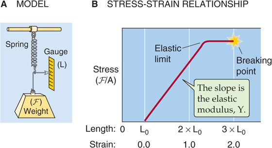
Figure 19-9 Elastic properties of a spring.

Stress is the force per unit cross-sectional area (F/A). Thus, if we pull on an elastic band—stretching it from an initial length L0 to a final length L—the stress is the force we apply, divided by the area of the band in cross section. Strain is the fractional increase in length, that is, ΔL/L0 or (L − L0)/L0 (Fig. 19-9B). An equation analogous to Hooke’s law describes the relationship between stress and strain:

The proportionality factor, Young’s elastic modulus (Y), is the force per cross-sectional area required to stretch the material to twice its initial length and also the slope of the strain-stress diagram in Figure 19-9B. Thus, the stiffer a material is, the steeper the slope, and the greater the elastic modulus. For example, collagen is more than 1000-fold stiffer than elastin (Table 19-5). (See Note: Young’s Modulus)

Table 19-5 Elastic Moduli (i.e., Stiffness) of Materials

* 1 mm Hg = 1334 dynes/cm2.

Because the elastic and collagen fibers in blood vessels are not arranged as simple linear springs, the stresses and strains that arise during the pressurization or filling of a vessel occur, at least in principle, along three axes (Fig. 19-10): (1) an elongation of the circumference (θ), (2) an elongation of the axial length (x), and (3) a compression of the thickness of the vessel wall in the direction of the radius (r). In fact, blood vessels actually change little in length during distention, and the thinning of the wall is usually not a major factor. Thus, we can describe the elastic properties of a vessel by considering only what happens along the circumference. (See Note: Axes of Vessel Deformation)

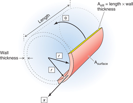
Figure 19-10 Three axes of deformation.

The transmural pressure (ΔP) is the distending force that tends to increase the circumference of the vessel. Opposing this elongation is a force inside the vessel wall. It is convenient to express this wall tension (T) as the force that must be applied to bring together the two edges of an imaginary slit, of unit length L, cut in the wall along the longitudinal axis of the vessel (Fig. 19-11). Note that in using tension (units: dynes/cm) rather than stress (units: dynes/cm2), we assume that the thickness of the vessel wall is constant.

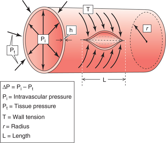
Figure 19-11 Laplace’s law. The circumferential arrows that attempt to bring together the edges of an imaginary slit along the length of the vessel represent the constricting force of the tension in the wall. The radial arrows that push the wall outward represent the distending force. At equilibrium, the two sets of forces balance.

The equilibrium between ΔP and T depends on the vessel radius and is expressed by a law derived independently by Thomas Young and Marquis de Laplace in the early 1800s. For a cylinder, (See Note: Laplace’s Law)

Thus, for a given transmural pressure, the wall tension in the vessel gets larger as the radius increases.

The vascular wall is adapted to withstand wall tension, not transmural pressure

In Figure 19-8, we plotted the volume of a vessel against transmural pressure, finding that the slope of this relationship is compliance. However, this sort of analysis does not provide us with direct information on the spring-like properties of the materials that make up the vessel wall. With Laplace’s law (T = ΔP · r), we can transform the pressure-volume relationship into the same kind of “elastic diagram” that we used in Figure 19-9B to understand the properties of a rubber band.

Figure 19-12A is a re-plot of the pressure-volume diagrams in Figure 19-8. In Figure 19-12B, we reverse the coordinate system so that volume is now on the x-axis and pressure on the y-axis. Finally, in Figure 19-12C, we convert volume to radius on the x-axis and use Laplace’s law to convert pressure into wall tension on the y-axis. The plots in Figure 19-12C are analogous to a stress-strain diagram for a rubber band (Fig. 19-9B). Thus, stretching the radius of the aorta (solid red curve) causes a considerable rise in wall tension, reflecting the aorta’s moderate compliance. The vena cava, on the other hand, fills over a wide range of radii before any wall tension develops, reflecting the shape change that makes it appear to be very compliant at the low pressures that are physiological for a vein. However, further stretching of the vein’s radius results in a steep rise in wall tension, reflecting the inherently limited compliance of veins. (See Note: Length-Tension vs Strain-Stress Diagrams)

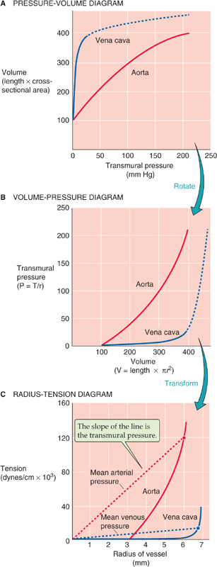
Figure 19-12 Elastic diagram (tension versus radius) of blood vessels. In A, the curves are re-plots of the curves in Figure 19-8. In B, the plot is the result of reversing the two axes in A. In C, the solid red and blue curves are transformations of the curves in B. If we solve for r, the x-axis of B (volume) becomes radius in C; if we use Laplace’s law (T = ΔP · r) to solve for T, the y-axis of B (transmural pressure) becomes tension in C.

What does Laplace’s law (Equation 19-8) tell us about the wall tension necessary to withstand the pressure inside a blood vessel? On the plot of tension versus radius for the aorta in Figure 19-12C, we have chosen a single point at a radius of 6 mm; because the aorta is relatively stiff, stretching it to this radius produces a wall tension of 120,000 dynes/cm. According to Laplace’s law, exactly one pressure—200,000 dynes/cm2 or 150 mm Hg—satisfies this combination of r and T. In Figure 19-12C, this pressure is indicated by the slope of the red broken line that connects the origin with our point. In a similar exercise for the vena cava, we assume a radius of ~6.7 mm, which is similar to the one we chose for the aorta; because the vena cava is readily deformed in this range, expanding it to this radius produces a wall tension of only 12,000 dynes/cm (blue broken line). This combination of r and T yields a much lower pressure—18,000 dynes/cm2, or 13.5 mm Hg. Thus, comparing vessels of similar size, Laplace’s law tells us that a high wall tension is required to withstand a high pressure.

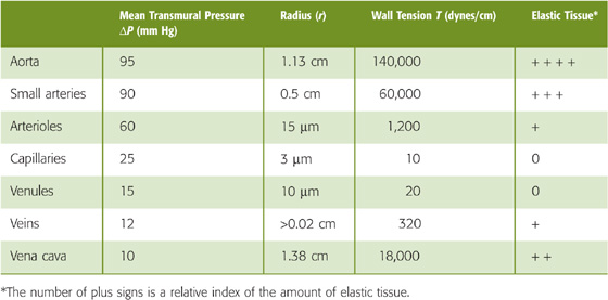
Comparing two vessels of very different size reveals a disparity between wall tension and pressure. A large vein, such as the vena cava, must resist only 10 mm Hg in transmural pressure but is equipped with a fair amount of elastic tissue. A capillary, on the other hand, which must resist a transmural pressure of 25 mm Hg, does not have any elastic tissue at all. Why? The key concept is that what the vessel really has to withstand is not pressure but wall tension. According to Laplace’s law (Equation 19-8), wall tension is the product of transmural pressure and radius (ΔP · r). Hence, wall tension in a capillary (10 dynes/cm) is much smaller than that in the vena cava (18,000 dynes/cm), even though the capillary is at a higher pressure. Table 19-6 shows that the amount of elastic tissue correlates extremely well with wall tension but very poorly with transmural pressure. The higher the tension that the vessel wall must bear, the greater is its complement of elastic tissue.

Table 19-6 Comparison of Wall Tensions and Elastic Tissue Content in Various Vessels

Elastin and collagen separately contribute to the wall tension of vessels

The solid red and blue curves in Figure 19-12C are quite different from the linear behavior predicted by Hooke’s law (Fig. 19-9B). With increasing stretch, the vessel wall resists additional deformation more; that is, the slope of the relationship becomes steeper. The increasing slope (i.e., increasing elastic modulus) of the radius-tension diagram of a blood vessel is due to the heterogeneity of the elastic material of the vascular wall. Elastic and collagen fibers have different elastic moduli (Table 19-5). We can quantitate the separate contributions of elastic and collagen fibers by “chemical dissection.” After selective digestion of elastin with elastase, which unmasks the behavior of collagen fibers, the length-tension relationship is very steep and closer to the linear relationship expected from Hooke’s law (Fig. 19-13, orange curve). After selective digestion of collagen fibers with formic acid, which unmasks the behavior of elastic fibers, the length-tension relationship is fairly flat (Fig. 19-13, blue curve). The orange curve (collagen) is steeper than the blue curve (elastin) because collagen is stiffer than elastin (Table 19-5). In a normal vessel (Fig. 19-13, red curve), modest degrees of stretch elongate primarily the elastin fibers along a relatively flat slope. Progressively greater degrees of stretch recruit collagen fibers, resulting in a steeper slope.

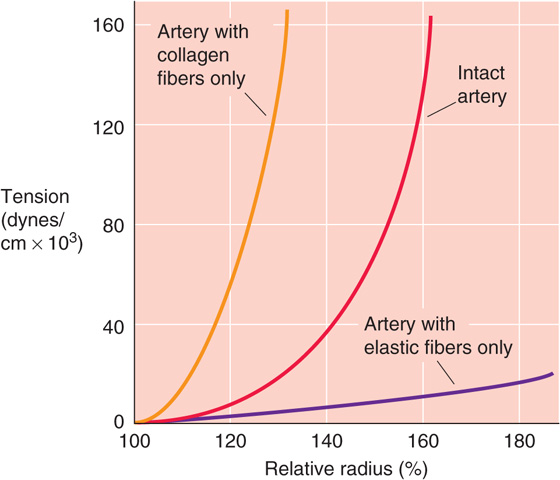
Figure 19-13 Chemical dissection of elastic moduli of collagen and elastin.

Aging reduces the distensibility of arteries

With aging, important changes occur in the elastic properties of blood vessels, primarily arteries. We can look at these age relationships for arteries from two perspectives, the pressure-volume curve and the radius-tension curve.

The most obvious difference in aortic pressure-volume curves with increasing age is that the curves shift to progressively higher volumes (Fig. 19-14A), reflecting an increase in diameter. In addition, the compliance of the aorta first rises during growth and development to early adulthood and then falls during later life. After early adulthood, two unfavorable changes occur. First, arteriosclerotic changes reduce the vessel’s compliance per se. Thus, during ventricular ejection, a normal-sized increase in aortic volume (ΔV) in a young adult produces a relatively small pulse pressure (ΔP) in the aorta. In contrast, the same change in aortic volume in an elderly individual produces a much larger pulse pressure. Second, because blood pressure frequently rises with age, the older person operates on a flatter portion of the pressure-volume curve, where the compliance is even lower than at lower pressures. Thus, a normal-sized increase in aortic volume produces an even larger pulse pressure.

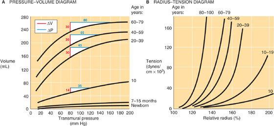
Figure 19-14 The effect of aging on arteries. In A and B, a relative radius of 100% represents the fully relaxed value. In A, the white triangles show the expected change in transmural pressure (blue line) for increase in aortic blood volume (red line) produced by each heartbeat—assuming a diastolic pressure of 80 mm Hg.

The second approach for assessment of the effects of age on the elastic properties of blood vessels is to examine the radius-tension diagram (Fig. 19-14B). Because of the progressive, diffuse fibrosis of vessel walls with age, and because of an increase in the amount of collagen, the maximal slope of the radius-tension diagram increases with age. In addition, with age, these curves start to bend upward at lower radii, as the same degree of stretch recruits a larger number of collagen fibers. Underlying this phenomenon is an increased cross-linking among collagen fibers (see Chapter 62) and thus less slack in their connections to other elements in the arterial wall. Thus, even modest elongations challenge the stiffer collagen fibers to stretch.

Active tension from smooth muscle activity adds to the elastic tension of vessels

Although we have been treating blood vessels as though their walls are purely elastic, the active tension (see Chapter 9) from VSMCs also contributes to wall tension. Stimulation of VSMCs can reduce the internal radius of muscular feed arteries by 20% to 50%. Laplace’s law (T = ΔP · r) tells us that as the VSMC shortens—thereby reducing vessel radius against a constant transmural pressure—there is a decrease in the tension that the muscle must exert to maintain that new, smaller radius.

For a blood vessel in which both passive elastic components and active smooth muscle components contribute to the total tension, the radius-tension relationship reflects the contributions of each. The red curve in Figure 19-15 shows such a compounded (passive + active) radius-tension diagram for an artery in which the sympathetic neurotransmitter norepinephrine (see Chapter 14) has maximally stimulated the VSMCs. The green curve shows a passive radius-tension relationship for just the elastic component of the tension (after the active component is eliminated by poisoning of the VSMCs with potassium cyanide). Of course, the green curve is the radius-tension diagram on which we have focused the previous figures (e.g., Fig. 19-12C). Subtraction of the green from the red curve in Figure 19-15 yields the active length-tension diagram (blue curve) for the vascular smooth muscle. (See Note: Stability of Vessels with Combined Active and Passive Tension)

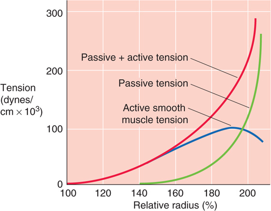
Figure 19-15 Active versus passive tension. The relative radius of 100% is that of an excised vessel maximally stimulated by norepinephrine (red curve, total tension) but not “stressed” (i.e., transmural pressure is 0). When the vessel is maximally poisoned with potassium cyanide, the baseline radius is approximately 150% (green curve, passive tension), reflecting its relaxed state. The blue curve is just the active (i.e., smooth muscle) component of tension.

Elastic tension helps stabilize vessels under vasomotor control

Consider a vessel initially stretched to a radius that is 80% greater than the unstressed radius (i.e., 180 versus 100 on the x-axis of Fig. 19-15). As we inject more fluid into the vessel, the radius increases (i.e., the vessel is more “stressed”). As a result, total wall tension must increase (Fig. 19-15, red curve). The opposite, of course, would happen if we were to withdraw some fluid from the vessel. During such changes in total wall tension, what are the individual contributions of vascular smooth muscle tension and the passive connective tissue tension? In Figure 19-16, we consider two extreme examples, one in which the vessel has only elastic elements and another in which it has only a fixed (i.e., isotonic) active tension.

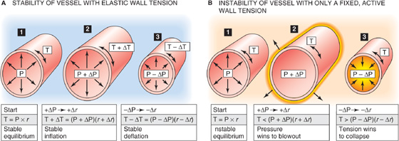
Figure 19-16 Mechanical stability of vessels.

First, consider a vessel lacking smooth muscle, so that only elastic elements contribute to total wall tension (Fig. 19-16A). If we increase transmural pressure from P (panel 1) to P + ΔP (panel 2), thereby increasing the radius from r to r + Δr, wall tension will automatically increase from T to T + ΔT. This increase in tension allows the vessel to reach a new equilibrium, according to Laplace’s law:

Conversely, a decrease in pressure must lead to a decrease in radius and a decrease in tension (panel 3). To achieve either the stable inflation of panel 2 or the stable deflation of panel 3, ΔT cannot be zero. In other words, the passive radius-tension diagram (Fig. 19-15, green curve) cannot have a slope of zero. The vessel wall must have some elasticity.

Second, consider a hypothetical case in which no elastic fibers are present and in which the total tension T is kept constant by active elements (i.e., VSMCs) alone. For example, this would be approximately the case for the blue curve in Figure 19-15, between relative radii of 180% and 200%. At the start (Fig. 19-16B, panel 1), we will assume that the smooth muscle tension exactly balances the P · r product. However, when we now increase pressure (panel 2), the automatic adaptation of tension that we saw in the previous example would not occur. Indeed, any increase in pressure would make the product (P + ΔP) · (r + Δr) exceed the fixed T of the VSMCs. As a result, the vessel would blow out. Conversely, any decrease in pressure would make the product (P − ΔP) · (r − Δr) fall below the fixed T and lead to full collapse of the vessel (panel 3). This type of instability does in fact occur in arteriovenous anastomoses, which are characterized by poor elastic tissue and abundant myoepithelioid cells.

A real vessel, whose wall contains both elastic and smooth muscle elements, can be stable (i.e., neither blown out nor collapsed) over a wide range of radii. The role of elastic tissue in vessels is therefore not only to withstand high transmural pressures but also to stabilize the vessel. Thus, elastic tissue ensures a graded response when smooth muscle tone changes. If vessels had only smooth muscle—and no elastic fibers—they would be like those in panels 2 and 3 of Figure 19-16B and tend to be either completely open or completely closed.

An imbalance between passive and active elastic components in blood vessels can be important in disease. For example, when the passive, elastic fibers of a blood vessel are reduced or damaged, vessels tend to become larger (e.g., aneurysms or varicosities). If the radius exceeds the value compatible with the physical equilibrium governed by Laplace’s law, a blowout may occur.

A second pathological example is seen when smooth muscle has undergone maximal stimulation and, conversely, passive elastic elements have regressed. This is the case in Raynaud disease, in which exposure to cold leads to extreme constriction of arterioles in the extremities, particularly the fingers. Vessel closure occurs because active smooth muscle tension dominates the radius-tension diagram.

REFERENCES