Chapter 11 Alternating current (AC) flow
Chapter contents
11.1 Aim
This chapter introduces the reader to alternating current (AC) flow. The various parameters used to measure such a current will be discussed. Simple AC circuits and three-phase power supplies will be considered.
11.2 Introduction
Direct current (DC) electricity (Ch. 7) is representative of a flow of electrons in one direction only. This chapter deals with the situation where electrons flow through a circuit first in one direction and then in the other (due to the changing polarity of the ends of the circuit) – this is known as an AC flow.
11.3 Types of DC and AC
Figure 11.1 shows different types of DC and AC in graphical form – the magnitude of the current (the dependent variable) is plotted on the vertical axis against time on the horizontal axis.
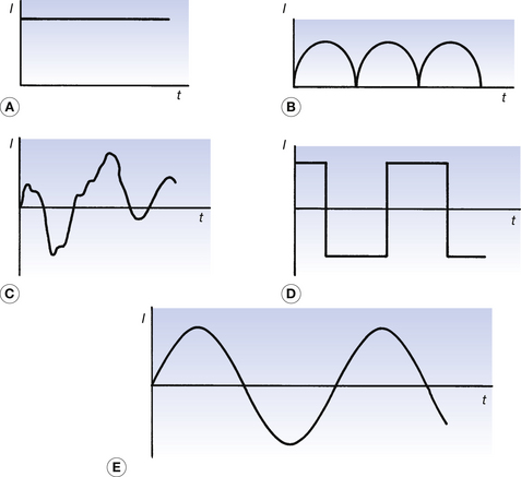
Figure 11.1 Types of direct current and alternating current: (A) constant DC; (B) pulsatile DC; (C) irregular AC; (D) square waveform AC; (E) sinusoidal AC.
Figure 11.1A is a case where the number of electrons passing a point per second in the circuit is constant producing a horizontal straight line. This is an example of the type of DC described in Chapter 7. Figure 11.1B is a case where the electrons always move in the same direction but the number of electrons passing a point varies with time – the electrons move as a series of pulses and this is known as pulsatable or pulsating DC. In Figure 11.1C there is no discernable pattern in the flow of electrons, except to say that they flow in both directions at different times. This is an example of an irregular AC waveform. Figure 11.1D shows a situation where the number of electrons travelling in one direction is constant for a short period of time and then the same number of electrons travel in the opposite direction for the same period of time. This is an example of a square waveform. Figure 11.1E shows an example of a sinusoidal AC wave form. This is the most common AC waveform and will be discussed in detail in the remainder of the chapter.
11.4 Sinusoidal AC
The sinusoidal AC waveform is shown in more detail in Figure 11.2, together with some of the quantities used to measure it.
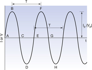
One cycle: One complete waveform starting at a point and continuing until the same point on the pattern is reached. This is usually measured from zero to zero (ABCDE) or from peak to peak (BCDEF).
Period (T): The time taken to complete one cycle, measured in seconds.
Frequency (f): The number of cycles which occur in 1 second, measured in cycles per second or hertz (Hz).
Amplitude: The maximum value of positive or negative current (or voltage) on the waveform. This may be referred to as the peak value.
There is a simple relationship between the period (T) and the frequency (f) which can be seen if we consider the following situation. Suppose we have a frequency of 10 Hz (10 cycles per second). Since the waveform is regular, each cycle must last for 0.1 second. Thus, we can say:

For a sinusoidal current, this equation may be rewritten as:

where It is the current at a time t and Ip is the amplitude or the peak value of the current. A similar equation can be produced for the voltage.
11.4.1 Peak current (or voltage)
The peak current is the same as the amplitude, i.e. it is the maximum positive or negative value of the current. Similarly, the peak voltage is the maximum value of the voltage. In radiography, the peak voltage across the tube, when the anode is positive and the cathode is negative, is usually quoted. If an X-ray tube is operating at 75 kVp then the peak potential difference between the anode and the cathode is 75 kV. The reasons for quoting the tube voltage as kVp will be considered later in this chapter.
11.4.2 Average current (or voltage)
As we can see from Figure 11.2, the average current flowing in one cycle of a sinusoidal waveform is zero, as the current flowing in one direction during the positive half-cycle has the same overall value (but of the opposite sign) during the negative half-cycle. The same conclusion applies to any number of complete cycles. A similar argument suggests that the average voltage for a sinusoidal waveform is also zero. Thus, for a sinusoidal waveform:

However, if the waveform is rectified (or made unidirectional; Ch. 28) then a value of the average current (or voltage) is obtained. The voltage waveform produced for half-wave rectification is shown in Figure 11.3A. This results in a pulsating voltage which (assuming a complete external circuit) results in a net electron flow in one direction – this allows us to consider average values of voltage and current which are not zero.
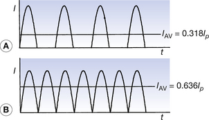
Figure 11.3 Forms of rectified sinusoidal alternating current: (A) half-wave rectification; (B) full-wave rectification.
The voltage waveform for a full-wave rectified circuit is shown on the same scale in Figure 11.3B. Again, a pulsating voltage is produced where the average value is twice that for the half-wave rectified circuit as there are twice as many peaks in unit time.
Thus, we can say for half-wave rectification:

and for full-wave rectification:

11.4.3 Effective (or RMS) current or voltage
If an AC supply is connected across a resistor, then electrons will flow in one direction during the first half-cycle and in the opposite direction during the second half-cycle. As there is no net movement of electrons for any given number of complete cycles, the average current is zero.
This does not mean that the net heating effect is zero. Electrons will produce heat within a resistor irrespective of their direction of travel. The average current is therefore a quantity, which is not suitable for determining the energy or power expended in a circuit which is connected to an AC supply. The quantity of importance is the effective or root mean square (RMS) value of the current and may be defined as:
The effective current is that value of constant current which, flowing for the same time, would produce the same expenditure of electrical energy in a circuit as the alternating current.
The effective value of the current is also known as the RMS value, for reasons which we will consider below. The effective or RMS voltage is defined in a very similar manner:
The effective voltage is that voltage which, being present for the same time, would produce the same expenditure of energy in a circuit as the alternating voltage.
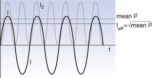
Consider the graphs shown in Figure 11.4. The AC I has an average value of zero because each positive value is matched by an equal and opposite negative value. Thus the peak positive value is matched with a peak negative value. If we take these peak values and square them, we can get rid of the negative sign and so it is possible to get an average value of the peak current (or voltage) squared. If we take the square root of this value, we now have the root of the mean of the square of the peak value. This is the effective value of the current (or voltage):

In Section 7.9.3 it was shown that the general equation for electrical power was W=V×I, where W is expressed in watts, V in volts and I in amperes. In an AC circuit, both V and I are constantly changing and so it is the effective or RMS value of each that must be taken into account when using the above equation:

Here, W is the average power generated in the circuit, taking into account at least one half-cycle of AC. We can manipulate Equation 11.5 in a similar way to Equation 7.16 to get:

Note: we can apply Ohm’s law (Ch. 7) to AC circuits provided the same types of units for voltage or current (e.g. RMS) are used throughout the equation.
The RMS values of current or voltage can be related to the peak relationships by the following equations:


Thus, for an AC, the effective value is just over 70% of the peak value.
11.5 AC and the X-RAY Tube
In order to produce X-rays, the X-ray tube requires a high potential difference (voltage) across it and a current flowing through it. The voltage available from the mains supply is far too low for use directly across the X-ray tube so a means of increasing it to the high values of thousands of volts is required. This is relatively easy to accomplish using an AC transformer (Ch. 14). Since this transformer increases the voltage, it is known as a step-up transformer. The filament of the X-ray tube requires a low voltage supply so that it can produce the electrons that form the mA through the tube, and so the mains voltage passes through a step-down transformer before being applied to the filament. Thus, an alternating voltage may either be increased using a step-up transformer or decreased using a step-down transformer.
In AC circuits, the voltages or currents are usually expressed in terms of their effective values unless otherwise stated. When considering the X-ray circuit, the following conventions apply:
• The voltage across the tube (kV) is expressed in terms of the peak voltage, i.e. kVp.
• The current flowing through the tube (mA) is expressed in terms of the average current.
• The mains voltage and current to the X-ray generator are expressed as effective or RMS values.
11.5.1 Voltage across the X-ray tube (kVp)
The potential difference across the X-ray tube is expressed in terms of the peak value for the following reasons:
• The maximum energy of X-ray photons emitted by the anode is the same value in keV, i.e. an X-ray tube operated at 100 kVp will emit X-ray photons with a maximum energy of 100 keV. (This will be explained in more detail in Ch. 21.)
• The voltage rating of the high-tension cables must be able to withstand the maximum voltage applied to them. This occurs during the peak value of the voltage.
If the voltage applied to the X-ray tube is a constant potential (Ch. 28), then this is effectively a DC supply so the peak and the effective values are the same.
11.5.2 Current through the X-ray tube (mA)
The mA display is designed to measure the average current flowing through the X-ray tube during an exposure. The intensity of the radiation beam is proportional to the average current. If we take the average current (mA) and multiply this by the exposure time in seconds, we get the mAs for that exposure. This represents the total charge that has passed through the X-ray tube during the exposure. The quantity of X-rays produced during the exposure is proportional to the mAs.
11.5.3 The mains voltage and current
The electrical mains is the source of power and so it makes sense to quote the mains supply in terms which make the calculations of power most convenient – the effective or RMS values. The mains voltage in the UK has a nominal value of 230 voltsRMS and so this gives us a peak value for this voltage of approximately 325 volts (Equation 11.8).
11.6 Basics of AC Circuits
Having considered the different measures that can be made of an alternating current or voltage, we are now ready to look at the consequences of passing this current through some basic circuits.
11.6.1 Phase difference
So far in this chapter we have only considered the case where the peak voltage occurs at the same time as the peak current. The current and voltage are then said to be in phase. This is not necessarily true for all types of AC circuits and we can get situations where a phase difference exists between the current and the voltage. Examples of phase differences are shown in graphical form in Figure 11.5. In Figure 11.5A, the current (I) lags behind the voltage (V) – a waveform displaced to the right occurs later than, and therefore lags behind, the waveform with which it is being compared. Also, in Figure 11.5B, we have a situation where I leads V.
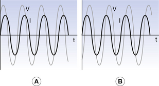
Figure 11.5 Phase differences between current and voltage waveforms: (A) I lags behind V; (B) I leads V.
The angle between the two waveforms is expressed as the phase angle where 360° is equivalent to one cycle.
11.6.2 Reactance and impedance
When we considered the opposition to the flow of direct current in a circuit, we found that this opposition consisted of resistance and was measured in ohms (see Ch. 7). There are two additional measures of AC resistance in a circuit: reactance and impedance. Both are measured in ohms as in DC resistance but measure different quantities.
To summarize, resistance, reactance and impedance all represent opposition to the flow of current and are all measured in ohms. They are expressed by the ratio of volts to amperes but the voltage vector is different in each case – it is in phase with the current for resistance, at right angles to the current for reactance and at the phase angle to the current for impedance. Impedance is thus the general term for opposition to current flow, and reactance and resistance form separate components of this.
11.7 Simple AC Circuits
In a simple AC circuit containing only resistance, the opposition to current flow rises through Ohm’s law which can be applied to calculate power consumption in the same way as in DC circuits. When capacitors and inductors are introduced in an AC circuit we need to consider the opposition to current flow caused by capacitors and inductors. This opposition, reactance, is in addition to the opposition to current flow rising from resistance.
The combination of resistance and reactance of an AC circuit, the impedance, can be calculated. However, these calculations can be quite complex and fall into the realm of electronic engineering, not radiography, and so will not be covered in any detail in this chapter.
11.8 Three-Phase AC
The basis of the generation of electricity was explained in Section 10.9. However, the requirements for electrical power vary widely depending on the machinery used. Any national electrical supply must be able to cope with a wide variation in the demand for electrical power. This is made possible by the winding geometry of three-phase AC generators. These have three symmetrical windings, making three phases of AC available as shown diagrammatically in Figure 11.6. The windings, W1, W2 and W3 in Figure 11.6A, are on a rotor, but are separated by an angle of 120° and, as the rotor is rotated, each winding moves through a magnetic field in turn.
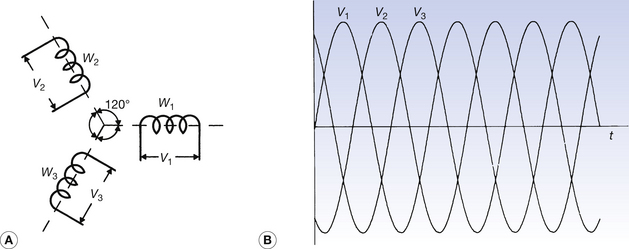
Figure 11.6 Three-phase electrical generation. (A) Diagrammatic representation of three sets of windings in the alternating current generator; (B) graphical representation of the three voltage phases against time showing the 120° separation between each phase.
Each set of windings has a sinusoidal alternating voltage induced in it (see Sect 10.9) but these voltages are out of phase with each other because of the different times they encounter the strongest regions of the magnetic field within the generator. These voltages (V1, V2 and V3 from the windings W1, W2 and W3) are known as phase voltages and are separated by 120° from each other, as shown in 11.6B. Thus a phase difference of 120° exists between each phase voltage. These voltages are now increased by the use of a step-up transformer for transmission over long distances and are then stepped down for use in industry, hospitals, homes, etc., using suitable star and delta connections of the phase voltages, as outlined below.
11.8.1 Star and delta connections
Star and delta connections of the phase voltages are shown in Figure 11.7. If we assume that an RMS voltage of 230 volts is induced in each winding of the generator, then three sets of 230-volts supply are available from the delta connection. The centre of the star connection is called the neutral and is kept as near earth potential as possible by equalizing the power outputs from the three phases. This allows the possibility of six voltages from the star connection:
• Three phase voltages of 230 volts are possible if a connection is made to the neutral and to one end of a winding.
• Three line voltages of 398 volts are possible by making connections to the ends of two of the windings – one such connection is shown between W1 and W3.
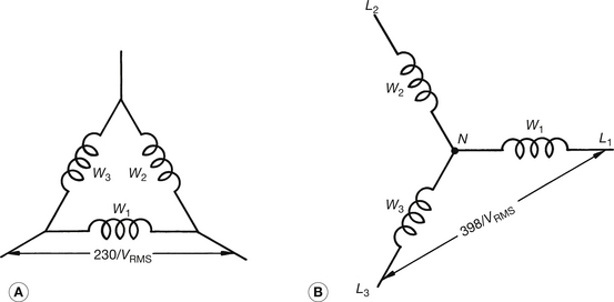
Note that the line voltage is 398 volts and not 460 volts as would be expected, as each phase voltage is 230 volts. This is because of the phase difference between the phase voltages. It may be shown (see Insight below) that the line voltage is also sinusoidal and has a magnitude which is a factor of √3 greater than the phase voltage.
The difference between the voltages across L1 and L3 in Figure 11.7 is the difference between the voltages across L1–N and L2–N. If we consider a situation where the potential of N is zero, L1–N is 10 volts and L3–N is 4 volts, then the potential difference between L1 and L3 is 10−4=6 volts. Thus, we may use the vector diagram shown in the Figure 11.8.
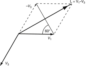
Thus the line voltage is √3 times the phase voltage. In the UK, the phase voltage is 230 volts (RMS) and so the line voltage is 398 volts (RMS).
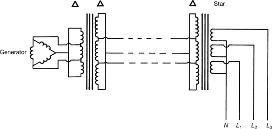
The transfer of power from the generating station to a city, which makes use of delta and delta transformers, is shown diagrammatically in Figure 11.9. The four wires L1, L2, L3 and N are distributed to domestic, hospital and industrial users and the appropriate voltages (phase or line) are available; phase voltages for domestic use and both phase and line voltages for hospital and industrial use. The star connection is often referred to as a three-phase four-wire supply, for obvious reasons.
11.8.2 Three-phase circuits in radiography
There are two main uses for three-phase supplies used in radiography:
1. The line voltage from a three-phase supply is used to ensure that a 398-volt supply is available for most static X-ray sets. This means that the turns ratio (see Ch. 14) required in step-up transformers is less than that required for a 230-volt supply.
2. The induction motor used to rotate the anode of the X-ray tube uses three phases. This is further discussed in Chapter 30.
In this chapter, you should have learnt the following:
• Sinusoidal AC is described mathematically by the formula I=Ip sin 2πft and V=Vp sin 2πft where Ip and Vp are the peak current and voltage and f is the frequency of the AC supply in hertz (see Sect. 11.4).
• One cycle is one complete waveform; the period is the time for one cycle; the frequency is the number of cycles per second; and the amplitude is the maximum value of voltage or current (see Sect. 11.4).
• The frequency (f) and the period (T) are related by the equation f=1/T (see Sect. 11.4).
• For a sinusoidal waveform, the average current (or voltage) is=0. For half-wave rectified AC, the average current (or voltage) is=0.318×peak current (voltage). For full-wave rectified AC, the average current (or voltage) is=0.636×peak current (voltage) (see Sect. 11.4.2).
• The definition of the RMS current as that value of constant current which, acting over the same time, would produce the same expenditure of electrical energy in a circuit as the AC. All AC voltages and currents are quoted in RMS values unless otherwise stated. IRMS=0.707×Ip; VRMS=0.707×Vp (see Sect. 11.4.3).
• Voltages across the X-ray tube are expressed in peak voltages (kVp); current through the tube is expressed in average value (mA), and mains supply is expressed in RMS values (see Sect. 11.5).
• Three-phase circuits consist of three sinusoidal waveforms 120° apart. These may be connected by star or delta configurations (see Sect. 11.8).
• The phase voltage is that across individual windings; the line voltage is that obtained across each of the three connections of the star and delta connections. For a delta connection, the line and phase voltages are equal; for a star connection, the line voltage is √3× the phase voltage (see Sect. 11.8.1).