Chapter Sixteen Correlation
Introduction
A fundamental aim of scientific and clinical research is to establish relationships between two or more sets of observations or variables. Finding such relationships or co-variations is often an initial step for identifying causal relationships.
The topic of correlation is concerned with expressing quantitatively the degree and direction of the relationship between variables. Correlations are useful in the health sciences in areas such as determining the validity and reliability of clinical measures (Ch. 12) or in expressing how health problems are related to crucial biological, behavioural or environmental factors (Ch. 5).
Correlation
Consider the following two statements:
You probably have a fair idea what the above two statements mean. The first statement implies that there is evidence that if you score high on one variable (cigarette smoking) you are likely to score high on the other variable (lung damage). The second statement describes the finding that scoring high on the variable ‘overweight’ tends to be associated with low measures on the variable ‘life expectancy’. The information missing from each of the statements is the numerical value for degree or magnitude of the association between the variables.
A correlation coefficient is a statistic which expresses numerically the magnitude and direction of the association between two variables.
In order to demonstrate that two variables are correlated, we must obtain measures of both variables for the same set of subjects or events. Let us look at an example to illustrate this point.
Assume that we are interested to see whether scores for anatomy examinations are correlated with scores for physiology. To keep the example simple, assume that there were only five (n = 5) students who sat for both examinations (see Table 16.1).
| Score (out of 10) | ||
|---|---|---|
| Student | Anatomy (X) | Physiology (Y ) |
| 1 | 3 | 2.5 |
| 2 | 4 | 3.5 |
| 3 | 1 | 0 |
| 4 | 8 | 6 |
| 5 | 2 | 1 |
To provide a visual representation of the relationship between the two variables, we can plot the above data on a scattergram. A scattergram is a graph of the paired scores for each subject on the two variables. By convention, we call one of the variables x and the other one y. It is evident from Figure 16.1 that there is a positive relationship between the two variables. That is, students who have high scores for anatomy (variable X) tend to have high scores for physiology (variable Y). Also, for this set of data we can fit a straight line in close approximation of the points on the scattergram. This line is referred to as a line of ‘best fit’. This topic is discussed in statistics under ‘linear regression’. In general, a variety of relationships is possible between two variables; the scattergrams in Figure 16.2 illustrate some of these.
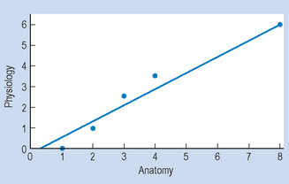
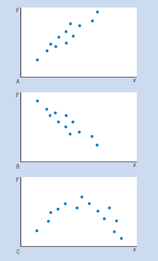
Figure 16.2 Scattergrams showing relationships between two variables: (A) positive linear correlation; (B) negative linear correlation; (C) non-linear correlation.
Figure 16.2A and B represent a linear correlation between the variables x and y. That is, a straight line is the most appropriate representation of the relationship between x and y. Figure 16.2C represents a non-linear correlation, where a curve best represents the relationship between x and y.
Figure 16.2A represents a positive correlation, indicating that high scores on x are related to high scores on y. For example, the relationship between cigarette smoking and lung damage is a positive correlation. Figure 16.2B represents a negative correlation, where high scores on x are associated with low scores on y. For example, the correlation between the variables ‘being overweight’ and ‘life expectancy’ is negative, meaning that the more you are overweight, the lower your life expectancy.
Correlation coefficients
When we need to know or express the numerical value of the correlation between x and y, we calculate a statistic called the correlation coefficient. The correlation coefficient expresses quantitatively the magnitude and direction of the correlation.
Selection of correlation coefficients
There are several types of correlation coefficients used in statistics. Table 16.2 shows some of these correlation coefficients, and the conditions under which they are used. As the table indicates, the scale of measurements used determines the selection of the appropriate correlation coefficient.
Table 16.2 Correlation coefficient
| Coefficient | Conditions where appropriate |
|---|---|
| φ (phi) | Both x and y measures on a nominal scale |
| ρ (rho) | Both x and y measures on, or transformed to, ordinal scales |
| r | Both x and y measures on an interval or ratio scale |
All of the correlation coefficients shown in Table 16.2 are appropriate for quantifying linear relationships between variables. There are other correlation coefficients, such as η (eta) which are used for quantifying non-linear relationships. However, the discussion of the use and calculation of all the correlation coefficients is beyond the scope of this text. Rather, we will examine only the commonly used Pearson’s r, and Spearman’s ρ (rho).
Regardless of which correlation coefficient we employ, these statistics share the following characteristics:
Calculation of correlation coefficients
Pearson’s r
We have already stated that Pearson’s r is the appropriate correlation coefficient when both variables x and y are measured on an interval or a ratio scale. Further assumptions in using r are that both variables x and y are normally distributed, and that we are describing a linear (rather than curvilinear) relationship.
Pearson’s r is a measure of the extent to which paired scores are correlated. To calculate r we need to represent the position of each paired score within its own distribution, so we convert each raw score to a z score. This transformation corrects for the two distributions x and y having different means and standard deviations. The formula for calculating Pearson’s r is:

where zx = standard score corresponding to any raw x score, zy = standard score corresponding to any raw y score, Σ = sum of standard score products and n = numbers of paired measurements.
Table 16.3 gives the calculations for the correlation coefficient for the data given in the earlier examination scores example.
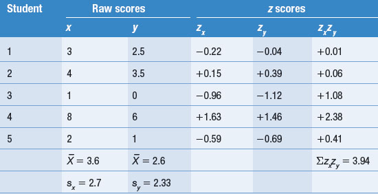
(The z scores are calculated as discussed in Ch. 15.)
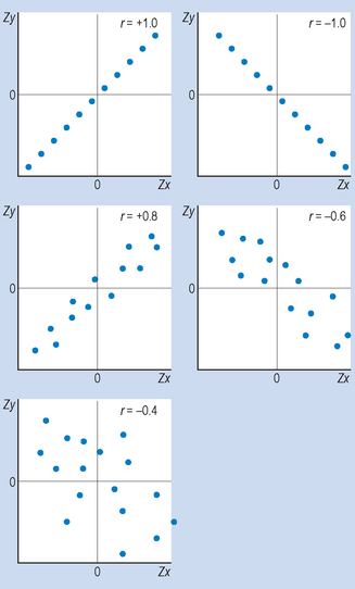
This is quite a high correlation, indicating that the paired z scores fall roughly on a straight line. In general, the closer the relationship between the two variables approximates a straight line, the more r approaches + 1. Note that in social and biological sciences correlations this high do not usually occur. In general, we consider anything over 0.7 to be quite high, 0.3–0.7 to be moderate and less than 0.3 to be weak. The scattergrams in Figure 16.3 illustrate this point.
When n is large, the above equation is inconvenient to use to calculate r. Here we are not concerned with calculating r with a large n, although appropriate formulae or computer programs are available. For example, Coates & Steed (2003, Chapter 5) described how to use the program ‘SPSS’ for calculating correlation coefficients. The printouts provide not only the value of the correlation coefficients but also the statistical significance of the associations.
Assumptions for using r
It was pointed out earlier that r is used when two variables are scaled on interval or ratio scales and when it is shown that they are linearly associated. In addition, the sets of scores on each variable should be approximately normally distributed.
If any of the above assumptions are violated, then the correlation coefficient might be spuriously low. Therefore, other correlation coefficients should be used to represent association between two variables. A further problem may arise from the truncation of the range of values in one or both of the variables. This occurs when the distributions greatly deviate from normal shapes. The higher scale can be readily reduced to an ordinal scale.
If we measure the correlation between examination scores and IQs of a group of health science students, we might find a low correlation because, by the time students present themselves to tertiary courses, most students with low IQs are eliminated. In this way, the distribution of IQs would not be normal but rather negatively skewed. In effect, the question of appropriate sampling is also relevant to correlations, as was outlined in Chapter 3.
Spearman’s ρ
When the obtained data are such that at least one of the variables x or y was measured on an ordinal scale and the other on an ordinal scale or higher, we use ρ to calculate the correlation between the two variables. The higher scale can be readily reduced to an ordinal scale.
If one or both variables were measured on a nominal scale, ρ is no longer appropriate as a statistic.
where d = difference in a pair of ranks and n = number of pairs.
The derivation of this formula will not be discussed here. The 6 is placed in the formula as a scaling device; it ensures that the possible range of ρ is from − 1 to + 1 and thus enables ρ and r to be compared. Let us consider an example to illustrate the use of ρ.
If an investigator is interested in the correlation between socioeconomic status and severity of respiratory illness, and assuming that both variables were measured on, or transformed to, an ordinal scale, the investigator rank-orders the scores from highest to lowest on each variable (Table 16.4).
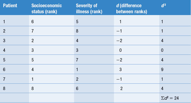
Clearly, the association among the ranks for the paired scores on the two variables becomes closer the more ρ approaches + 1. If the ranks tend to be inverse, then ρ approaches − 1.
Uses of correlation in the health sciences
Prediction
When the correlation coefficient has been calculated it may be used to predict the value of one variable (y) given the value of the other variable (x). For instance, take a hypothetical example that the correlation between cigarette smoking and lung damage is r = + 1. We can see from Figure 16.4 that, given any score on x, we can transform this into a z score (zx) and then using the graph we can read off the corresponding z score on y (zy). Of course, it is extremely rare that there should be a perfect (r = + 1) correlation between two variables. In this case, the smaller the correlation coefficient, the greater the probability of making an error in prediction. For example, consider Figure 16.5, where the scattergram shown represents a hypothetical correlation of approximately r = 0.7. Here, for any transformed value on variable x (say Zx1) there is a range of values of zy that correspond. Our best guess here is Zy1, the average value, but clearly a range of scores is possible, as shown on the figure.
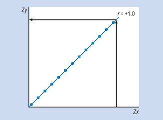
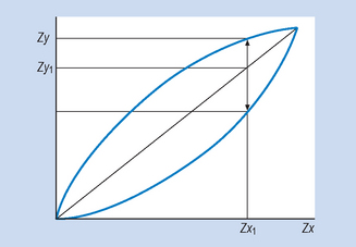
Figure 16.5 Hypothetical relationship between cigarette smoking and lung damage. r = + 0.7. With a correlation of <1.0 the data points will cluster around rather than exactly on the line and may vary between the range of values shown for any given values of x or y and their corresponding z scores.
That is, as the correlation coefficient approaches 0, the range of error in prediction increases. A more appropriate and precise way of making predictions is in terms of regression analysis, but this topic is not covered in this introductory book.
Reliability and predictive validity of assessment
As you will recall, reliability refers to measurements using instruments or to subjective judgments remaining relatively the same on repeated administration (Ch. 12). This is called test–retest reliability and its degree is measured by a correlation coefficient. The correlation coefficient can also be used to determine the degree of inter-observer reliability.
As an example, assume that we are interested in the inter-observer reliability for two neurologists who are assessing patients for degrees of functional disability following spinal cord damage. Table 16.5 represents a set of hypothetical results of their independent assessment of the same set of five patients.
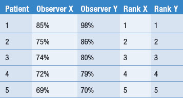
Observer Y clearly attributes greater degrees of disability to the patients than observer X. However, as stated earlier, this need not affect the correlation coefficient. If we treat the measurement as an ordinal scale, we can see from Table 16.5 that the ranks given to the patients by the two observers correspond, so that it can be shown that ρ = + 1.
Clearly, the higher the correlation, the greater the reliability. If we had treated the measurements as representing interval or ratio data, we would have calculated Pearson’s r to represent quantitatively the reliability of the measurement.
Predictive validity is also expressed as a correlation coefficient. For example, say that you devise an assessment procedure to predict how much people will benefit from a rehabilitation programme. If the correlation between the assessment and a measure of the success of the rehabilitation programme is high (say 0.7 or 0.8), the assessment procedure has high predictive validity. If, however, the correlation is low (say 0.3 or 0.4), the predictive validity of the assessment is low, and it would be unwise to use the assessment as a screening procedure for the entry of patients into the rehabilitation programme.
Estimating shared variance
A useful statistic is the square of the correlation coefficient (r2) which represents the proportion of variance in one variable accounted for by the other. This is called the coefficient of determination.
If, for example, the correlation between variable x (height) and variable y (weight) is r = 0.7, then the coefficient of determination is r2 = 0.49 or 49%. This means that 49% of the variability of weight can be accounted for in terms of height. You might ask, what about the other 51% of the variability? This would be accounted for by other factors, say for instance, a tendency to eat fatty foods. The point here is that even a relatively high correlation coefficient (r = 0.7) accounts for less than 50% of the variability.
This is a difficult concept, so it might be worth remembering that ‘variability’ (see Ch. 14) refers to how scores are spread out about the mean. That is, as in the above example, some people will be heavy, some average, some light. So we can account for 49% of the total variability of weight (x) in terms of height (y) if r = 0.7. The other 51% can be explained in terms of other factors, such as somatotype. The greater the correlation coefficient, the greater the coefficient of determination, and the more the variability in y can be accounted for in terms of x.
Correlation and causation
In Chapter 4, we pointed out that there were at least three criteria for establishing a causal relationship. Correlation or co-variation is only one of these criteria. We have already discussed in Chapter 6 that even a high correlation between two variables does not necessarily imply a causal relationship. That is, there are a variety of plausible explanations for finding a correlation. As an example, let us take cigarette smoking (x) and lung damage (y). A high positive correlation could result from any of the following circumstances:
For the example above, (1) would imply that cigarette smoking causes lung damage, (2) that lung damage causes cigarette smoking, and (3) that there was a variable (e.g. stress) which caused both increased smoking and lung damage. We need further information to identify which of the competing hypotheses is most plausible.
Some associations between variables are completely spurious (4). For example, there might be a correlation between the amount of margarine consumed and the number of cases of influenza over a period of time in a community, but each of the two events might have entirely different, unrelated causes. Also, some correlation coefficients do not reach statistical significance, that is, they may be due to chance (see Chs 18 and 19).
Also, if we are using a sample to estimate the correlation in a population, we must be certain that the outcome is not due to biased sampling or sampling error. That is, the investigator needs to show that a correlation coefficient is statistically significant and not just due to random sampling error. We will look at the concept of statistical significance in the next chapter.
While demonstrating correlation does not establish causality, we can use correlations as a source for subsequent hypotheses. For instance, in this example, work on carcinogens in cigarette tars and the causes of emphysema has confirmed that it is probably true that smoking does, in fact, cause lung damage (x causes y). However, given that there is often multiple causation of health problems, option (3) cannot be ruled out.
Techniques are available which can, under favourable conditions, enable investigators to use correlations as a basis for distinguishing between competing plausible hypotheses. One such technique, called path analysis, involves postulating a probable temporal sequence of events and then establishing a correlation between them. This technique was borrowed from systems theory and has been applied in areas of clinical research, such as epidemiology.
Summary
In this chapter we outlined how the degree and direction between two variables can be quantified using statistics called correlation coefficients. Of the correlation coefficients, the use of two were outlined: Pearson’s r and Spearman’s ρ. Definitional formulae and simple calculations were presented, with the understanding that more complex calculations of correlation coefficients are done with computers.
Several uses for r and ρ were discussed: for prediction, for quantifying the reliability and validity of measurements, and by using r2 in estimating amount of shared variability. Finally, we discussed the caution necessary in causal interpretation of correlation coefficients. Showing a strong association between variables is an important step towards establishing causal links but further evidence is required to decide the direction of causality.
As with other descriptive statistics, caution is necessary when correlation coefficients are calculated for a sample and then generalized to a population. The question of generalization from a sample statistic to a population parameter will be discussed in the following chapters.
Self-assessment
Explain the meaning of the following terms:
True or false
Multiple choice
| Test | Test–retest reliability (r) | Predictive validity (r) |
|---|---|---|
| P | 0.8 | 0.50 |
| Q | 0.9 | 0.18 |
| R | 0.5 | 0.40 |
| S | 0.2 | 0.03 |
